Hansen Solubility Parameters in Practice (HSPiP) e-Book Contents
(How to buy HSPiP)
Chapter 11,
Cracks in the system (Environmental Stress
Cracking)
It’s not every day that you are asked to
solve a very expensive problem for a large aquarium. A fire had damaged the
large PMMA front of the shark tank for a famous aquarium. Replacing such a
large piece of PMMA would have been very expensive. But it was unthinkable to
risk having it fail whilst full of water and sharks. With the aid of a few
drops of liquid and a deep understanding of HSP and environmental stress
cracking (ESC), one of us (Hansen) was able to say authoritatively that the
tank was entirely fit for purpose – a decision vindicated by many years
of safe use since it was refilled.
We’ll discuss a rather simpler example in
this chapter, but it’s good to know that the principles can be applied to many
different situations, including large shark tanks.
ESC is a huge practical problem. It is said
that at least 25% of failures in plastics are caused by it. Almost by
definition it is a difficult problem. Yet HSP can very quickly tell you if you
are likely to be in an ESC danger zone.
Let’s remind ourselves of the problem. You
have a polymer part that you don’t want to be damaged by contact with solvent.
So you do some tests with a range of solvents. If you try a good solvent (i.e.
inside the sphere of the polymer) then, yes, you have a problem in that the
polymer dissolves. But really this isn’t a serious problem. The test takes a
few moments and you then know that you must keep that solvent away from that
polymer part. If the part has to handle
that solvent then you have to change the polymer. With a solvent you know to be
outside the sphere you know the answer in advance but you do the test anyway and,
of course, the solvent doesn’t do anything to the plastic. It will not be a
problem, so you say that this solvent is safe to use.
And yet, some days, months, years later
after exposure to this “safe” solvent the plastic suddenly cracks and you have
an expensive repair bill or an angry customer. Where had you gone wrong? The
answer is in the thermodynamics. You’d rightly concluded that there was a net
increase in energy if the solvent infiltrated the polymer and therefore it
would not interact. What you’d forgotten was the “S” in ESC. The stress is
another factor that can tip the thermodynamic balance. If you have a large
concentration of stress, and if the solvent and polymer are near the
thermodynamic tipping point then the solvent can enter the plastic and, snap,
you have your cracked or broken part.
When the problem is expressed in these
terms, the solution is obvious. You will only get ESC from solvents that are
near the border of the sphere. Solvents inside give dissolution and you easily
identify them. Solvents far outside will never be close to the thermodynamic
limit and will therefore never cause ESC. So for those of us who have to worry
about ESC the rule is simple: Beware of solvents at the boundary – and
therefore make sure you know where your boundary is.
Here is a typical example based on the
Topas 6013 ESC example in the Handbook.
For this plot, only true solvents were used
to define the HSP
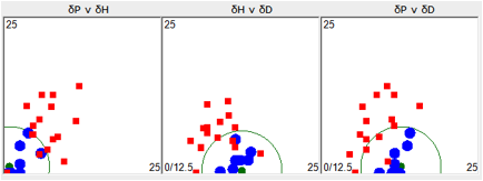
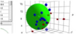
Figure 1‑1 Using file ESC with “Inside” set to 1
This doesn’t tell you much about ESC.
For the next plot, solvents that tended to
show ESC are included in “Inside”. The calculated HSP and radius has changed.
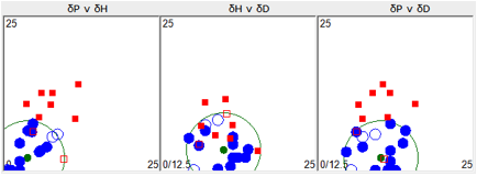
Figure 1‑2 Using file ESC with “Inside” set to 2
The point of this plot is that the solvents
outside this radius are almost certain to be safe from ESC.
The “almost” is there for two good reasons.
First, the radius defining ESC depends strongly on the Stress. If the stress is
low, then the radius is close to the first plot. If the stress is high then the
ESC radius will expand. Only you can judge the level of stress and therefore
the margin of safety for solvents. Second, the molar volume plays a role.
Smaller molecules are able to diffuse more easily into the polymer and
contribute to the weakening of the polymer and potential cracking. So when you
form your judgement on whether a solvent outside the radius is safe, err on the
side of caution if that solvent is small.
Stressing
“stress”
It’s important to stress the “stress” part
of ESC. At a high enough stress a polymer will crack even with a
poorly-compatible solvent. An excellent paper to illustrate this point is C. H.
M. Jacques and M. G. Wyzgoski, Prediction
of Environmental Stress Cracking of Polycarbonate from Solubility
Considerations, Journal of Applied Polymer Science, 23, 1153-1166, 1979. PC
parts were stressed to different extents and placed in test solvents. In each
case there was a critical stress above which the part would crack. For
obviously good solvents such as toluene, the critical stress was low
(<0.3%), for obviously bad solvents such as ethylene glycol the stress was
high (>1.9%).
One way of looking at these data come from
Hansen’s review of HSP and ESC, Charles M. Hansen, On predicting environmental stress cracking in polymers, Polymer
Degradation and Stability, 77, 2002, 43–53. First the HSP sphere is
calculated not on the basis of solubility but on how much strain is needed
before the PC cracks in solvent. In the re-work of that data (including some
corrections to the data from other papers) the Sphere comes out at a surprising
[21.9, 10.2, 5.2, 13.8]. But remember that this is a Sphere based on ESC not on
solubility for which the radius, and presumably the HSP will be rather
different. For reasons that will become clear in a moment this is forced to be
[21, 7.6, 4.4, 10.2] for further data analysis. Hansen then plotted the RED
number v Molar Volume for these solvents, dividing the plot into classes
depending on whether they required low, medium or high strains before cracking.
Here is a simplified version of the original graph, using the revised data:
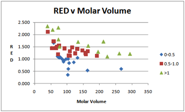
Figure 1‑3 RED v Molar Volume for the PC ESC data file
Not surprisingly, there is a general
correlation between low RED number and low strains before cracking. But what is
also clear is that low molar volume solvents must be further away from the PC
(i.e. higher RED number) – in other words, for a given RED number, small
molecules give more stress cracking.
In
a graph (not shown) of RED v strain required to crack, there is a
general trend (as expected) that high RED requires high strain. But the fit is
very poor. Instead, a fitted trend was created using a combination of RED and
Molar Volume. It turns out that the best fit comes from RED * MVol0.333.
And the best fit was found with the
HSP values mentioned above.
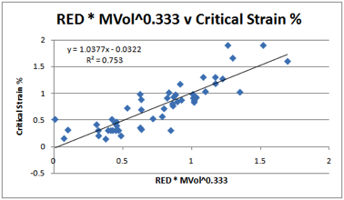
Figure 1‑4 PC Critical Strains % correlated with RED and MVol0.333
Clearly the correlation isn’t perfect. Nor
should it be. For example a detailed analysis in the Jaques’ paper shows (as we
would expect) that branched hydrocarbons require a higher critical strain than
unbranched equivalents because (as discussed in the Diffusion chapter) branched
solvents diffuse more slowly.
Similar plots can be produced from the %
strain data of other polymers. For Polysulfone (not shown) there is a similar
good fit to a 0.333 dependency on MVol. However, for PMMA and PPO there are big
differences:
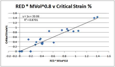
Figure 1‑5 PMMA Critical Strains % correlated with RED and MVol0.8
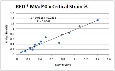
Figure 1‑6 PPO Critical Strains % correlated with RED and MVol0
On the basis of these four polymers a
tentative conclusion can be reached about the MVol effect. The Sphere radii for
the four fits are: PMMA 8, PC/PSF 10.5, PPO 13.5. It seems reasonable (though
of course it is unproven without considerably more experimental data) that for
polymers with large radii (PPO), the ease of molecular access is high so the
MVol effects are small. Conversely, for polymers with smaller radii (PMMA)
there is a far greater specificity and therefore a larger dependence on MVol.
For the ESC predictor described below we have set up a MVol dependency varying
from a minimum of 0 at 13 and above linearly up to a (fitted and meaningless)
value of 2.2 at a radius of 0. This means that a Sphere of radius 7 has a
linear dependency on MVol.
Readers will be unhappy with the tentative
nature of the above. But those who wish to criticise should first consider the
amount of work required to get good data. First there is the basic experimental
data. It is thankless and dull work to get data over a sufficiently large range
of solvents that span both the HSP space and also MVol space. Only two of the
correlations feature molecules with MVol > 150 so it is hard to get
statistically meaningful fits. Second there is comment from these authors that
there is no substitute for the original data. Some of the values for some of
the polymers quoted in some secondary literatures are just plain wrong. It was
a sobering experience to spend the time entering data from the secondary
literature, getting absurd plots, then discovering that the data had been
misquoted.
For old polymers there may be no reason to
re-do the ESC data as the user community more or less know which solvents to
avoid for long-term use. But with so many new bio-polymers coming on the market
it would seem a good idea to invest the time and energy producing critical
strain data. Although it is a lot of effort, compared to the consequences of an
unexpected failure out in the real world it would seem to be a good investment
of scientific time.
Because users of HSPiP wanted an ESC
predictor we have provided what we call an ESC guide. Because ESC depends on
HSP, on MVol, on branched/unbranched solvent shapes, on stress and (sometimes)
on surface stress it’s simply not possible to provide a complete ESC predictor.
Instead we’ve provided a colour-coded guide that follows the rainbow. The
colours are based on the combination of RED and MVolx, where the
power x varies from 2.2 to 0 between a radius of 0 and 13. The larger the
Sphere the more solvents will be caught in the ESC trap, so it’s important that
you know what your sphere is based on. If it’s based on solubility then it will
tend to be on the small side. If it’s based on a critical stress value then it’s
more likely to be realistic. Red and yellow are for molecules usually well
inside the Sphere. These will probably not cause ESC simply because they will
obviously damage the polymer in early tests. Such solvents have been known to
give ESC, however, when they have been found in aqueous mixtures even at very
small concentrations. If the water can evaporate, the solvent concentration can
become very high, and ESC has been found. Greens will tend to be around the
border so should be prone to ESC. Blues will tend to be far-enough away to
provide low ESC probabilities. But remember that if the stress is large enough
almost any solvent can cause ESC.
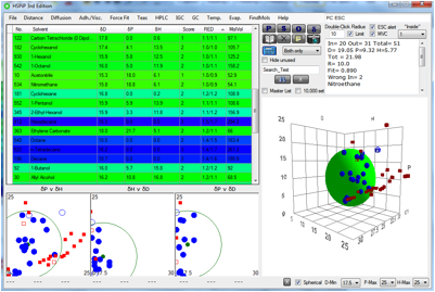
Figure 1‑7 ESC colour-coding taking into account MVol as well as RED. Blue is
typically safer than green. The data shown are in the middle of the range.
It’s therefore up to you to use the colour
guide as a guide.
To summarize: to avoid ESC make sure that
the solvents used are well outside the Sphere and have a large molar volume
and, if possible, branched, low diffusion shape. If your polymer will encounter
larger stresses then the solvents will have to be further outside the sphere
with an even larger molar volume. On the polymer side it is known that
incorporation of a smaller amount of higher molecular weight polymer (bimodal)
vastly improves stress cracking resistance, while still allowing for acceptable
processing conditions. This is reminiscent of the phenomena discussed early on
adhesion and polymer chain entanglement. The intimate mixing of polymers having
widely different molecular weights is possible by simultaneous use of two
different catalysts for polyethylene, for example.
These theoretical considerations can be
illuminated by some practical examples encountered by Hansen. ESC with PC has
been found on evaporating insulin solutions stabilized with 0.15% m-Cresol.
There are also examples of surfactants in automotive windscreen cleaners that
have cracked PC parts on the car. Then there is the classic of the stick-on
label on a PC helmet giving ESC. An example of ESC with serious environmental
consequences arose several years after the gluing of a PVC joint. There was a
little piece of a rag in the threading that over time gave enough stress to
initiate the crack. The PVC near the rag failed in a mode that started with
stringing polymer, which meant solvent in some quantity was present, and this
then extended through the whole joint and gave an environmental catastrophe
since strong base in a large amount got into a nearby stream. This was a large
media event at the time, and all because a solvent wiping rag was able to
initiate ESC.
E-Book contents | HSP User's Forum