Hansen Solubility Parameters in Practice (HSPiP) e-Book Contents
(How to buy HSPiP)
Chapter 12
Let’s make this perfectly clear
… (Formulating
clear automotive lacquers)
If you are trying to make a hard, clear
coating a good starting point would be an isocyanate cross-linked polyol
system. There are many isocyanates, many polyols and therefore it is a
straightforward process to create a formulation with the right balance of
pot-life, cure speed, cross-link density, hardness, scratch resistance etc.
The final desirable feature, clarity/gloss,
requires the whole cross-linking and drying process to take place without any
phase-separation of any of the components. This isn’t as easy as it sounds.
It’s likely that a solvent blend is used, for the right balance of solubility,
drying rate, health and safety, as discussed previously. The problem is that a
solvent blend which might have been good for the starting isocyanate and polyol
may not be good for the polymer as it forms. Or even if that blend were OK, the
fact that the different components evaporate at different speeds means that the
solubility parameters are changing, perhaps for the better or perhaps for the
worse.
Formulating such a coating by trial and
error is therefore very hard work. As the authors know from personal
experience, formulating with the help of HSP makes the task much easier and,
ultimately, more profitable.
In this book we use real-world examples as
much as possible, but in this case we will merely be illustrative. Readers
should be able to extend the principle to their own situation.
For an isocyanate we’ll use TDI, Tolylene
diisocyanate. For a polyol we will use an oligomeric hydroxyl-propyl
methacrylate. The HSP for TDI are known, [19.3, 7.9, 6.1] Using S-P group
contributions (see the DIY chapter for what S-P means) the oligomer can be
estimated as [16, 10, 12]. The polymer can similarly be estimated as [18, 11, 7].
In this simple analysis we can choose to ignore
the issue of dissolving the TDI as it is a liquid at the presumed 25ºC for
making our basic formulation. So our problem is to have a solvent which is
excellent for the oligomer and which becomes excellent for the polymer.
If we go to the solvent optimizer our first
task is to find a “friendly” solvent with a sufficiently high δH without it
containing any –OH functionality which would interfere with the
cross-linking reaction. We also need this to be relatively volatile as we want
the δH component to drop significantly during the curing/drying process.
By Ctrl-clicking on the solvents containing
alcohols (or creating a “friendly solvent” list without alcohols) it is
relatively easy to find that a 69:31 mixture of PMA (Propyleneglycol
Monomethylether Acetate) and GBL (Gamma ButyroLactone) is an adequate fit,
though not surprisingly the δH is rather lower than desirable. But as it’s only
an oligomer we are trying to dissolve, its radius will be rather large so this
mix should be OK.
The HSP of that mixture are [16.3, 9.0, 9.1].
For our polymer we clearly need a
significant increase in δD. The GBL is less volatile than PMA and has a high δD so we’re off to a good
start, but the δP is very high. So we need something to bring that down. DBE
(DiBasic Ester) is low boiling and as a 57:43 mix with GBL is quite close to
our polymer at [17.2, 11.5, 7.8].
So now we need to work out a blend of PMA
with DBE and GBL to get the best possible compromise. A 75:14:11 mix of PMA,
GBL and DBE gives [16.0, 7.0, 9.3], a distance of 4 from the oligomer. This
seems adequate.
Now we need to check how the solvent blend
changes with time. The relative evaporation rates are PMA:GBL:DBE = 30:3:1. Within
the Solvent Optimizer there’s the option to model the evaporation. Here’s the
output from this particular simulation:
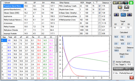
Figure 1‑1 Change in composition in time as the solvents evaporate. The setup
can be loaded as PerfectlyClear.sof
At the end of this simulation, the total
solvent (Blue data/graph) has decreased to 12% of its original amount. The PMA
(Red data/graph) decreased rapidly from 75 to <5% after a short time. Because
cross-linking reactions tend to slow down with time, we can guess that a good
deal of the cross-linking has taken place in that time, so the removal of the
PMA by that time is about right. The PMA:GBL (Green):DBE (Magenta) ratio at that
point is approximately 4:49:47, giving [17.1, 10.6, 8.9] (the HSP of the mix is
calculated for you in the simulation) a respectable distance of 2 from the polymer.
The ratio of GBL to DBE gradually shifted because of the factor of 3 in their
relative evaporation rates. Clearly the starting ratio should be changed to
reflect this if the resulting level doesn’t quite give the required
compatibility with polymer.
The high level of the low boilers at the
end of the curing reaction means that a final bake will be required, but this
would be required anyway as removal of the final % solvent becomes constrained
by diffusion rather than evaporation. The bake will also complete the
cross-linking reaction.
Note that in this run we’ve chosen to
include the effect of Activity Coefficients – when the presence of one
solvent increases the evaporation rate relative to another. To do this the
Activity Coefficients are calculated from the HSP distance between one solvent
and another (or one solvent and the HSP of the rest of the blend). The
calculation is based on the “enthalpic deviation from ideality” term involving
the χ parameter. For
solvent-solvent interactions one often-used formula is:
Equ. 1‑1 lnγ = ln (φ1/x1)
+ HSPDistance2 φ22*0.6MVol1/RT
For solvent-polymer interactions (an option
in the calculations) there is an additional term. To avoid over-complicating
the calculations, this second formula is used for all the interactions, on the
grounds that the errors in the assumptions will tend to balance out.
Responsibility for the use of this method is Abbott’s.
Equ. 1‑2 lnγ = ln (φ1/x1)
+ 1- φ1/x1 + HSPDistance2 φ22*0.6MVol1/RT
where φ is the volume fraction, x is the mole
fraction and γ is the activity coefficient. With solvents that are very close,
γ approaches 1, for solvents that are far apart γ might rise to 2 or 3 and, at
very low concentrations might rise as high as 10. These formulae and a warning
about the full complexity of multi-solvent/polymer calculations are found in J.
Holten-Andersen, C.M. Hansen, Solvent and
Water Evaporation from Coatings, Progress in Organic Coatings, 11, 219-240,
1983.
You can choose to include the Target
polymer in the activity coefficient calculations.
You can even do the calculations at an
elevated temperature. The relative evaporation rates are calculated by an
approximate fit (from Abbott: RER=0.046*MVol*VP) to the calculated vapour
pressures using Antoine Coefficients which are included for as many of the
Optimizer Solvents as possible. This seems to give a better fit over the range
of data than a published method (Stratta,
J. John, Dillon, Paul W., and Semp, Robert H., Evaporation of Organic Cosolvents from Water-borne Formulations.
Theory, Experimental Study, Computer Simulation, Journal of Coating
Technology, 50, 1978, 39-47) which has RER=0.822*MWt ½*VP.
Equ. 1‑3 RER = 0.046 MVol.
VapourPressure (mm Hg)
At the same time, the temperature
correction of HSP is also performed.
Here are the same 3 solvents at 50ºC
instead of the nominal 25ºC of the previous plot:
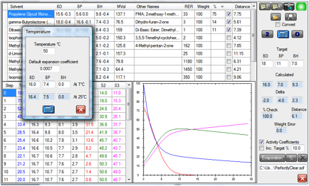
Figure 1‑2 The same system at 50ºC
Note that no meaningful Antoine
Coefficients (AA, AB, AC) are available for DBE as it’s a mixture so the values
were taken from DPG which has a similar RER at room temperature.
It’s likely that you will disagree with us
on the precise choice of solvent blend. And you’ll note that this simulation
says nothing about absolute time. It can’t – all it knows about is
relative evaporation rates. The modeller automatically adjusts itself so that
the fall-off of solvent at the start isn’t too rapid or too slow and the rest
of the curves then fit around that. Only you know what air flows you are
applying and whether the temperature of the drying system is lowered by
evaporative cooling. Both factors affect the absolute drying time. (For the 3rd
Edition we’ve let you do an absolute time calculation by specifying how long it
would take nBuAc to evaporate under your conditions.) But the point is that we
reached our decision via a rational process, with a “better than nothing” model
and when our coating isn’t quite as glossy as we would like, or our solvent
blend is a bit too expensive, or the level of residual solvent is a bit too
high, the formulation can be tweaked rationally.
What would have been the alternative? We
know the answer from real-world experience. The alternative is a lot of trial
and error, a lot of confusion, and the expenditure of a great deal of time and
energy.
We have to make a really important point
about the temperature corrections used for the optimization. You notice that
the HSP of all the solvents are changed by the temperature. This is mostly a
thermal expansion effect – the MVol increases with increasing
temperature. Why did we not change the HSP of the target? If, for example, the
solvent blend is a good match at room temperature, it’s possible that it will
be a bad match at a higher temperature. Exactly so! In a series of important
papers in the 1960s, Patterson repeatedly pointed out the existence of the LCST
“Lower Critical Solution Temperature”. This, confusingly (don’t blame us for
this mad nomenclature), is at a higher temperature than the UCST “Upper
Critical Solution Temperature”. The UCST comes from the 1/RT effect in the Chi
parameter and means that polymers are less soluble at lower temperatures. No
surprises there. The LCST is less familiar – the fact that polymers
(especially high MWt ones) start to become less soluble at higher temperatures
and eventually come out of solution. The explanation for this non-intuitive
effect lies exactly in the phenomenon we’re discussing. The HSP of the solvents
generally decrease with temperature because of thermal expansion. But the
polymer expansion coefficient is much smaller than that of the solvent so its
HSP stays approximately constant. So a perfect HSP match at room temperature
can become a large mismatch at high temperatures.
Don’t
blush
This is a good point at which to introduce
the new Blushing Estimator in the 3rd Edition. A solvent mix which
gives an excellent coating on a dry day might give a horrible coating on a day
with high relative humidity (RH). Or it might be OK if you dry slowly but
horrible if you increase the air flow to dry a bit faster. The reason is that
the evaporation of the solvent removes heat from the solution, causing it to
cool. If the surface temperature falls below the dew point of the air then
water can condense out, causing the coating defect often called “blushing”. The
dew point increases on days with high RH, and a faster air flow increases the
rate of evaporation and therefore lowers the surface temperature. Either of
these effects might tip the balance between a good and a blushed coating.
If you increase the airflow to the coating
you increase the rate of evaporation, which cools the coating further, which
then decreases the rate of evaporation. Clearly there is a point at which the
two effects balance out. This is the so-called Wet Bulb temperature of the
solution. If there’s sufficient heat coming in (e.g. via the substrate) or if the
air flow is not high enough, then the solution may be above the wet bulb
temperature. But it will never be below it. The web bulb temperature is the
worse-case scenario.
HSPiP has all the necessary data for the
calculation. From the HSP we know (by definition!) the enthalpy of
vapourisation. We also provide the Antoine Coefficients for a large range of
solvents – and Y-MB provides estimates for other solvents. The Antoine
Coefficients give the vapour pressures of the various components. Finally the
MVol is needed for knowledge of the actual (as opposed to molar) amount of
vapour in the air.
The wet bulb temperature is therefore
automatically calculated for any mix where all the data are known. By entering
the RH of the air we can also calculate the dew point of that air. If the dew
point is higher than the web bulb then the wet bulb value is surrounded by red
to give you a visual warning of the possibility of blushing.
Only you can tell whether the air flow is
low enough or the supply of heat from other sources is high enough to overcome
the blushing. But at least you have a quick way to check whether you are at
risk from blushing.
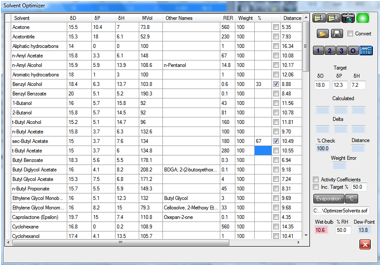
Figure 1‑3 This 67:33 blend of s-butyl acetate and benzyl alcohol has a wet-bulb
temperature below the current dew point of 13.8 degrees – so there is a
danger of blushing. Swapping the ratio of the solvents or reducing the RH to
40% (not shown) removes the possibility of blushing.
E-Book contents | HSP User's Forum