Chapter 13 , That’s swell (HSP and  Swelling)

If you look in the polymer data table you can find the same polymer giving different values. This can be deeply troubling to a first-time user and seems to undermine the whole premise of HSP.

Further thought reveals that some polymers must show different HSP under different conditions. This is such an important principle that we give it a chapter to itself.

For first-time users we provide an “Instant Guide” set of values for common polymers. Until you’ve built up your own experience, use these values for the polymers – but remember that they are only there as an instant guide and that other values might apply for your specific problem, as this chapter emphasises.

Let’s take for example PCTFE, PolyChloroTriFluoroEthylene.

If you calculate a sphere using data from solvents that swell it by >2% you get (though with so few good solvents, the fit is somewhat arbitrary) [17.9, 2.9, 2.7], typical of a C-Cl polymer:

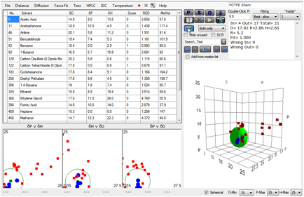
Figure 1‑1 A correlation with PCTFE swelling at 2% absorption

But if you do a plot with those solvents that swell by >5% you also get a very different good fit, typical of C-F polymers [15.6, 4.9, 7.5].

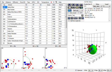
Figure 1‑2 Same polymer, different correlation at 5% absorption

What’s happening is that at low levels of solvent absorption, the solvents associate themselves with the –Cl rich areas of the polymer. As you go to greater swelling, the solvents have to associate with the predominant C-F regions.

This must be a general principle. If you test a polymer which contains a small portion of –OH functionality then at low levels of swelling, alcohols will be very happy to be associated with these regions, so the solvent sphere is biased towards the alcohol region. But when you start swelling/dissolving the whole of the polymer, the alcohols are very poor solvents, so the sphere shifts towards a lower δH and δP region.

Similarly, if a polymer contains crystalline and non-crystalline regions, then swelling data at low levels of solvent will reflect the non-crystalline region and therefore a bias towards whatever functionalities preferentially reside in that region.

So we can now flip the problem of having different solvent spheres into a distinct advantage. If you find conflicts in the data, these may well be providing you with fundamental insights into the internal structure of the polymer. It’s not obvious that PCTFE should have chlorine-rich and fluorine-rich regions, but the HSP data seem to suggest that that is the case.

The same principles can be applied to the latest nano-scale issues. It is becoming common practice to e-beam write nanostructures for integrated circuits, photonic crystals and nanobiology. When “negative” resists are used (i.e. those that become less soluble on exposure) there is a problem of development. You want a solvent that quickly whisks away the un-crosslinked resin. But such a solvent can readily enter the cross-linked polymer and cause it to swell. If you write 10nm features, then it only needs swelling of 5nm across both sides of the feature and the swollen polymers touch across the divide and degrade the quality of the image. One proposal to fix this is to use solvents just at the edge of the HSP sphere – they will still dissolve the un-crosslinked resin, but will be unlikely to enter the crosslinked system. We are grateful to Dr Deirdre Olynick and her team at Lawrence Berkeley National Laboratory for allowing us to reproduce data from their paper that explores these issues in a profound way: Deirdre L. Olynick, Paul D. Ashby, Mark D. Lewis, Timothy Jen, Haoren Lu, J. Alexander Liddle, Weilun Chao, The Link Between Nanoscale Feature Development in a Negative Resist and the Hansen Solubility Sphere, Journal of Polymer Science: Part B: Polymer Physics, Vol. 47, 2091–2105 (2009).

The team first established the HSP sphere for the calixarene resist of interest.

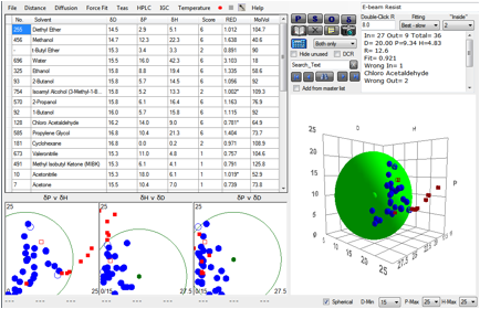
Figure 1‑3 Sphere for Calixarene e-beam resist

It is interesting to note that they used a sophisticated Sphere algorithm (fully described in their paper) which included some heuristics that could eliminate false fits. Happily, the values of our straightforward algorithm match theirs. They were then able to show that solvents closer to the centre of the sphere were better at creating high contrast images, whilst those near the edge were better at avoiding the problems caused by swelling. A rational compromise can then be reached on this basis. Importantly, other solvents and/or solvent blends can then easily be devised on rational principles to improve the process even further. The paper contains much more of interest and readers are recommended to explore their paper in detail.

Of course kinetics must be part of the optimisation process and it is likely that issues discussed in the Diffusion chapter will also play a part in understanding. But by establishing the basic thermodynamics of the system, further optimization can be a more rational process.

 

E-Book contents | HSP User's Forum