The sense of smell is still something of a mystery. But there are determined efforts to remove that mystery and there’s a good chance that HSP can play their part.

Professor William Goddard’s group at CalTech provides a good example of how HSP can be used to investigate both artificial and natural noses. Along the way, the group is also providing new tools for calculating HSP. We are grateful to Professor Goddard and his colleague Dr Mario Blanco for giving us access to their data and insights.

The artificial nose

A fruitful approach to producing an artificial nose is to provide a sensor made up of an array of sub-sensors each of which has a different response to an odorant molecule. Whilst the response from any individual sub-sensor might not tell you too much about an odorant, the “fingerprint” of responses might be sufficiently unique to tell you what odorant is there and how much of it is present.

The “JPL Artificial Nose” works in this way. There are seven sub-sensors, each a simple polymer: Poly(methylmethacrylate) (PMMA), Poly(4-hydroxystyrene) (P4HS), Polyethyleneoxide (PEO), Polyethylene (PE), Poly(ethylenevinyl acetate) (PEVA), Polysulfone, and Polycaprolactone.

The hypothesis of the Goddard group is that the amount of interaction (and therefore sub-sensor signal) of an odorant molecule could be predicted on the basis of its HSP distance from each polymer. Their work is described in their paper (in collaboration with 3M) M. Belmares, M. Blanco, W. A. Goddard III, R. B. Ross, G. Caldwell, S.-H. Chou, J. Pham, P. M. Olofson, Cristina Thomas, Hildebrand and Hansen Solubility Parameters from Molecular Dynamics with Applications to Electronic Nose Polymer Sensors, J Comput. Chem. 25: 1814–1826, 2004. Their analysis is based on their calculated HSP values from molecular dynamics. In this account we use conventional HSP for the simple reason that the paper’s values for δP and δH are necessarily constrained by the absence of an agreed methodology for producing these values from the MD data. We are grateful for their permission to recast the data in our mode and we must stress our enthusiasm for the MD approach where it is surely only a matter of time before the δP/δH problem is solved.

The aim of the paper was to see if there is a linear relationship between theoretical and experimental response curve. The logic is that the sensor response depends on swelling of the polymer by the solvent and the closer the solvent is to the HSP of the polymer the more swelling will occur. The fit was based on 5 parameters: a pre-exponential term, a term relating to molar volume, then a term each for the absolute differences of the cohesive energy terms values (polymer – solvent) of D, P and H.

Equ. 1‑1 Response = P1 * Exp(-P2*MV)*Exp(P3*(δDp-δDs) + P4*(δPp-δPs) + P5*(δHp-δHs))

We decided to see what happened if we used pure HSP instead. In that case we have just 3 parameters: the pre-exponential term, the molar volume term and term relating to the standard HSP distance.

Equ. 1‑2 Response = P1 * Exp(-P2*MV)*Exp(P3*Sqrt(4*(δDp-δDs)² + (δPp-δPs)² + (δHp-δHs)²))

The results are interesting and encouraging. With reasonable values for the δD, δP and δH values of the polymers, the fits were better (both in terms of slope and R²) than in the original paper. This isn’t as good as it sounds. The paper used the computed values and produced an honest fit. Because we had no direct knowledge of the polymers used we could “tweak” the polymer parameters (within reasonable limits) to get a good fit. To a certain extent we could argue (see the section on Chromatography) that this is a good way to derive HSP for polymers, but there is rather too much circularity in that argument.

Data from two of the polymers seem to be illuminating:

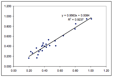
Figure 1‑1 Fit from the paper for the Polysulfone data using 5 fitting parameters

 

Figure 1‑2 Fit of the Polysulfone data using the HSP formulation and 3 parameters

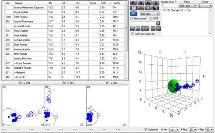
Figure 1‑3 Using file NoseChems and a Polysulfone of [15.4, 4.5, 2.8] There’s a reasonable mixture of overlapping and non-overlapping solvents, giving an overall wide-ranging response

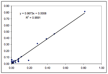
Figure 1‑4 For P4HS there is a less uniform response in the 5-parameter fit

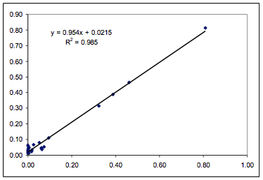
Figure 1‑5 With a slightly better, but still skewed fit from 3 parameters

 

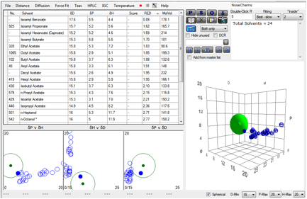
Figure 1‑6 With P4HS [18,8,2] there is very little polymer/solvent overlap, so it’s not surprising that most responses are clustered near one end of a rather small response curve

So at the very least the “pure” HSP approach looks interesting. And the fact that 3 parameters suffice to fit the experimental data from 24 solvents (using standard, un-tweaked HSP) with 7 polymers in a complex artificial nose is at the very least encouraging.

Natural noses

We don’t want to get involved in the major debates on how real noses manage to distinguish between so many different aromas. But it seems reasonable to most people that unless the aroma molecule has some affinity for a receptor site then that site won’t be able to detect it. And as soon as the word “affinity” is mentioned, it becomes natural to ask whether HSP could be a significant part of that affinity, and therefore a significant predictor of smell. We say “significant” because it is unrealistic to expect that every receptor is simply HSP generic. We are all familiar with the fact that biological receptors can be exquisitely specific (especially when it comes to optical isomers). So it seems reasonable that there will be elements of specificity in nasal receptors. But what seems to be clear is that no model based strongly on biological-style specificity has proven to be of general utility.

So how might one show that HSP can be insightful for understanding olfaction? The hypothesis from Blanco and Goddard (BG) is elegantly simple. For consistency with the rest of the book (and the eNose example above) we recast their hypothesis (with their permission) in a slightly different formulation but the effect is the same. They used Mean Field Theory (MFT) as their descriptor but we can think of it as HSP theory.

The BG-HSP hypothesis

Professor Linda Buck won the Nobel prize for identifying 47 different olfactory receptors. The BG-HSP hypothesis states that each of these olfactory receptors is defined by a δD, δP, δH and Radius as if it were a polymer. The response of each receptor to an odorant depends on the HSP distance of the odorant from the receptor.

Thus the Response_jk of receptor k to odorant j is given by

Equ. 1‑3 Response_jk = S_k * Exp(-a_k*Sqrt(4*(δDk-δDj)² + (δPk-δPj)² + (δHk-δHj)²))

which you will recognise as being almost identical to the eNose formula above – without the molar volume term. The formula can be made even more familiar with one simple change:

Equ. 1‑4 Response_jk = S_k * Exp(-Sqrt(4*(δDk-δDj)² + (δPk-δPj)² + (δHk-δHj)²)/R_k)

where we have replaced a_k with the more familiar Radius term R_k – so that the response has decreased by a factor of 1/e by the time the HSP distance is equal to R_k.

The beauty of this formula is that it can readily be tested and BG have provided the first HSP values for olfactory receptors.

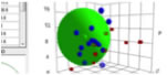
The response of the S19 receptor to 19 odorants is shown. The Sphere fit gives the HSP for S19 to be ~ [16.3, 5.5, 8.5].

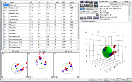
Figure 1‑7 Using file OlfactionS19

The S83 receptor gives: [16.4, 4.7, 8.4]:

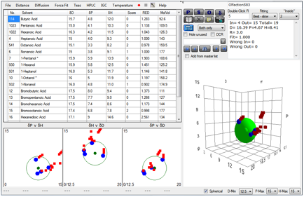
Figure 1‑8 Using file OlfactionS83

The process can be repeated for the other receptors. Note that the S83 receptor is more specific (R=3) than the S19 receptor (R=4).

When you try these examples out for yourself you will quickly find that we have shown the best possible interpretation of these data. The data sets are too small to provide good fits and it would be a massive task to take on such a vast project.

But as the original BG paper shows, the idea is, at the very least, a very fertile one. If olfaction is, as they guesstimate, 65% HSP and 35% specific receptor, then there will be plenty of noise in the data, but the HSP signal should shine through if the hypothesis is correct. And of course, life can be more complicated. Perhaps (and BG have evidence for this) some receptors have two HSP sites. A single Sphere fit would not do a good job so a more sophisticated multi-Sphere calculator would be required.

The reason the BG-HSP hypothesis is so important is because if it were shown to be true it would not be yet-another-correlation but a deep insight into olfactory receptors. Given that HSP are calculable ab-initio from molecular dynamics, and given that HSP represent fundamental thermodynamics, then olfaction (to, say, 65%) would become calculable from first principles.

If by the time you read this book the ongoing research has confirmed BG-HSP then we will be pleased that we spotted the significance of the BG research before it had reached maturity. If it has been disconfirmed then we’re pleased in another sense. For HSP to be good science it has to withstand the harsh standard of disconfirmation. If it has proven to have failed on such a big task as olfaction it at least had the merit of offering a clear prediction which could be refuted, and that’s one of the hallmarks of good science.

The Atlas of Odor Character Profiles

The Atlas, by Andrew Dravnieks, published by ASTM, ISDN 0-8031-0456-1, is a book of tables. For 144 odour chemicals plus a few more odour mixtures it lists to what extent a panel of skilled testers would say that each chemical smelled like X, where X was a list of 146 different odour sensations such as Fruity, Almond, Molasses, Yeasty, Incense, Kerosene, Sweaty, Heavy – to take a random cross-section through that list of sensations.

In the spirit of making refutable predictions, it seemed a good idea to assemble the HSP of all 144 chemicals then see how these fitted to the odour profiles. Of the 144 chemicals, many were in the standard Hansen table, but most were not. Thanks to the generosity of SC Johnson, a list of HSPs of 288 odour chemicals (prepared using calculation/estimation only by Charles Hansen) was made publicly available. This still left quite a few of the 144 without HSP so Abbott used the DIY-HSP tools from HSPiP to estimate the remaining ones. Both the SC Johnson list and the 144 list are made available as a contribution to further research on odours and fragrances. The 144 list includes CAS Numbers and Smiles notation to help you make sure which chemical is being referred to - naming of odorants is rather uncertain. Note that there are some minor errors in the Atlas. Where possible the table contains revisions to these errors.

Matching chemicals to the different sensations was made possible thanks to further tables in the Atlas. These listed the 5 highest-scoring chemicals for each sensation. The “minimum HSP sphere” that enclosed these 5 chemicals was then used as an indication of the hypothetical HSP centre/radius for each of these sensations.

Of course there are many problems with this procedure. First, some of the top 5 chemicals were from the mixtures which have not been included in the HSP list. Second, some of the “top 5” have such low scores as to make it seem unlikely that these sensations really do have well-defined chemical correlations. Third, the choice of 5 is rather arbitrary. If the size of responses (where a large number means a strong response) go (43, 41, 38, 34, 11) should that 5^th chemical (clearly much less relevant than the other four) be included? Or if the responses went (43, 41, 38, 34, 30, 29, 28, 11) shouldn’t we include the top 7 chemicals?

But we have to start somewhere. We’re only trying to explore some basic hypotheses. Others can feel free to refine the process if it seems to be worthwhile.

Although it was a lot of work, the “easy” part of the process was to identify the HSP centre/radius for each relevant sensation. The raw data are provided for you to save you the tedium of creating it for yourself. There were 70 aromas with meaningful high scores for which the centres of the minimum spheres were calculated.

Here is a screenshot from HSPiP showing 71 aromas in HSP space:

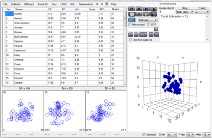
Figure 1‑9 Using file AromaScores

The hard part is working out whether the data mean anything. The simplest case would be that each sensation had a unique sensor which had a unique HSP for optimal binding. It’s obvious that aromas cannot work this way. Some of the sensations must be complex mixes of different sub-sensations. And the most optimistic HSP case would be that HSP compatibility is necessary but not sufficient – there must be a good HSP match for a molecule to be happy in the sensor area, but there must be other molecule-specific attributes for the aroma to register with the sensor.

An alternative would be to follow the process of A.M. Mamlouka, C. Chee-Ruiter, U.G. Hofmann, J.M. Bower, Quantifying olfactory perception: mapping olfactory perception space by using multidimensional scaling and self-organizing maps, Neurocomputing 52–54, 2003, 591 – 597. For those who are familiar with multidimensional scaling and self-organizing maps the data from our explorations are provided. However, the best that Abbott could do was to prepare a spreadsheet with a 71x71 matrix that calculated the HSP distance between each of the aromas. It was then possible to sort each column to see if the ordering of the aromas made sense. For example, if the target aroma was “bananas” which is arguably a pleasant aroma, other pleasant aromas might be expected to be close by and disgusting odours would be far away.

There was, unfortunately, no compelling evidence for this happy outcome. Here is a small section of the matrix ordered by distance between Banana and other aromas. Some of the fruity odours are gratifyingly close to Banana, but Urine and Rancid are also fairly close and they are not normally associated with the aroma of Banana.

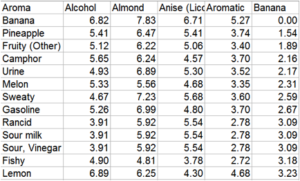
Figure 1‑10 A portion of the matrix ordered by the HSP distance between Banana and the other 70 odours.

Hansen published a paper in 1997 (Hansen, C.M., Aromastoffers Opløselighedsparametre (in Danish), Solubility Parameters for Aromas and Scents. Plus Process, 11, 16-17,1997) which anticipated many of these ideas. Readers may or may not like to know that it is possible to cover the smell of skatole (faeces) with suitably chosen (i.e. a good HSP match) aromas from hamburgers or bacon.

3^rd Edition update

With the benefit of hindsight, some of the ideas above do look naive. But it still seems to us that the world of fragrances is missing a trick by not taking HSP into account.

At the very least, the packaging industry could get a lot of benefit from the ideas of HSP and diffusion. If there is a good HSP match of a key fragrance/flavour component, say, Cinnamon (cinnamaldehyde) with a packaging polymer (such as poly lactic acid, PLA) then it’s highly likely that the polymer will be a poor barrier for it.

Similarly, if a fragrance component (or, more likely, fragrance formulation) has a good match for the HSP of skin then it’s more likely to penetrate the skin and (most likely) be lost as an odour.

And clearly if a fragrance/flavour component is to be delivered within some polymeric system (e.g. scratchable spheres) classic HSP calculations will help ensure a balance of good compatibility for creating the system and poor compatibility to ensure that the fragrance remains locked in to the system till required.

Because Sigma Aldrich have provided a de-facto standard reference for aromas, with helpful designation of the different types of smell, we are putting into the public domain an HSPiP version of the Sigma Aldrich Flavors & Fragrances catalogue. This is a somewhat error-prone undertaking as anyone who has ever handled complex datasets will know from their own experience. The catalogue doesn’t always provide CAS numbers and it doesn’t supply the Smiles. So at times we used the also excellent GoodScentsCompany website and you might find some alternative names for the same compound. We also had to decide what to include. Although we could have included the “W” numbers from the catalogue, there are so many variants of essentially the same compound that we decided it would not be helpful. Similarly, we could have provided the aroma class, but that would have created much duplication. From the name and/or the CAS number you should be able to identify most of the chemicals in the catalogue and therefore their aroma class. Finally, of course, we could not include those aromas that are mixtures and sometimes even the wonderful ChemSpider could not help us identify the right Smiles for a given compound. Nevertheless, you now have access to the HSP of over 800 aroma chemicals which you can then cross-reference with the Sigma Aldrich catalogue for your own purposes.

When you load it into HSPiP you will see the usual HSP data. But the horizontal scroll bar will allow you to scan across for the Smiles, CAS number etc. To search within the data you can try using a name (probably a truncated version as naming is so variable) or a CAS number.

One way of exploring whether HSP have any relation to aromas is via a Self Organising Map (SOM). Hiroshi has enjoyed playing with this concept and the following section shows the sort of exploration that can be done. It’s included as an indication of what might be done if someone wanted to throw some serious resource at the issue.

10 Fragrant Flowers

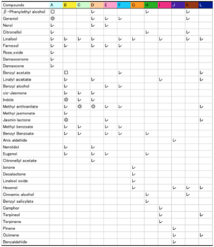
A Japanese website http://www001.upp.so-net.ne.jp/iromizu/hana_kaori_for_so-net.html lists the key ingredients of 10 flowers:

From the HSP of these molecules, and the different fragrances, an SOM can be constructed on a 40x40 matrix:

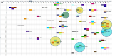
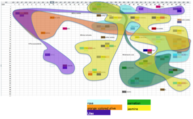
From this partition it’s possible to ask many questions. A typical one is “can we distinguish some key distinct notes from this?” And here’s one answer. 5 distinct areas stand out: Rose, Orange-colour olive, Lilac, Carnation and Jasmine stand out.

 

On the other hand, Ixora, Narcissus, Jasmine are rather similar in SOM space:

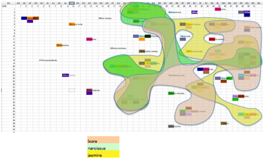
As we’re not trained in fragrances we can’t comment on the significance of these plots. But it represents another way of looking at how fragrances and solubilities may be related. If they show no relationship, that’s useful to know. If there are such relationships (and the physiology suggests that there should be) then HSP provide an opportunity for data mining in this fascinating area.

 

E-Book contents | HSP User's Forum