Chapter 32, Improvements?  

We’ve never tried to hide the imperfections of HSP. And we’ve often mentioned that we were working hard to create improved techniques. This chapter describes some of the outcomes of lots of hard work challenging our own assumptions.

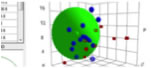
Sphere fitting

The official Sphere method described in the Handbook has served the HSP community very well for many years. There have been a few tweaks to it as HSPiP developed and a GA (Genetic Algorithm) method was added that coped better with some poor data sets. But now there are some logical alternatives to what we’ll now call the Classic method.

The first is a response to many users’ requests and something we had also wanted to do. It creates a Sphere based on real data which record, say, solubilities or swellabilities. In this case “more” is “better” – unless you choose the “good is small” option in which case “more” is “worse”. We had been greatly worried by the fact that the fitting algorithm would depend heavily on the assumptions behind the fit, and that neither we nor the user would know what those assumptions should be. But in the end we found that our worries were not necessary. The GA technique seems to do an excellent job fitting all sorts of  data. The centre of the Sphere is likely to be more accurate than an Inside/Outside fit, but the radius is unknown and has to be judged by yourself. You can do a simple check on this by selecting a “Split” value that defines “good” above it and “bad” below it.

The second is also something requested by users: a double sphere option that tries to find out if your sample contains a mixture of materials as in, for example, a di-block copolymer. The first thing to emphasise is caution. Fitting too little data with too many parameters can lead to too many errors. Finding objective criteria for finding the best of all possible pairs of Spheres is difficult and the GA works very hard to come up with a credible answer, but it can only do so much. So don’t get too excited about the two Spheres unless you are convinced that the data really does support the values.

MVol effects

It’s always been clear that smaller molecules should give higher solubility than their HSP distance might imply. The MVC option was an attempt to correct for this effect and some users (including ourselves) have found it helpful. In the Expert mode there is also a MVol option. The need for it has been tested by Hiroshi using his SOM (Self Organising Map) technique. With good data sets the SOM readily splits into two groups representing inside and outside. But with difficult sets, adding MVol as a parameter clearly helps to create a better split. Therefore MVol should give better Sphere data.

If this is true in general, it raises the question of how the Classic Sphere technique has ever been of much use. Such a question is even more relevant when we discuss Donor/Acceptor, so we’ll ask the question now, and provide a surprising answer.

Why has the Classic Sphere technique worked so well for so many years?

We were having a furious debate about Donor/Acceptor  and into the mix we threw the question of the MVol effect. It seemed to us that if these effects were significant then the Classic technique must have been wrong for all these years. From this we thought that either Donor/Acceptor or MVol effects must always be small, so that Classic was always right, or that the effects could be significant but somehow didn’t mess up the Classic fit. It was then we reached our “aha moment”. The majority of “good” solvents tend to sit in the middle of the Sphere. So if they are made a little better or a little worse by other effects then they would still be inside the Sphere and would make no difference to the fit. The same applies to the majority of “bad” solvents – if they are made a little better or worse by the effects then they would still be bad. The result is that the centre of the Sphere will not be changed much by any of these effects. The effects will change things on the border but that will mostly affect the radius. But we all know that the radius is not well defined anyway – it depends on the user’s judgement of what is “good” or “bad”. The same polymer could have very different radii if one user was concerned about solubility and another by swelling.

Turning this on its head, the fact that Classic HSP have worked so well for so many years demonstrates that Donor/Acceptor and MVol effects must be modest at best. For MVol corrections it turns out that a typical variation will be in the range of root-2. Theory suggests that MVol affects Distance² and if we say that a typical solvent has a MVol of 100, other solvents in the tests won’t range much below 50 or above 200. And in the next chapter we will find a plausible reason why Donor/Acceptor effects are usually irrelevant.

E-Book contents | HSP User's Forum