Utilities:

 

The Utilities use as common:

Screen Capture   

Table Capture 

Clear Button

Calculation Button 

 

Screen Capture    

 

For a permanent record, click Capture Screen to Clipboard.

 

You can then paste the image into Word etc. If you do Ctrl-Click you capture just the 3D image. If you do Shift-Click you capture just the 3 2D images. The Tooltip on the button reminds you of which option is which.

 

Table Capture  

For a permanent text record of the solvents, their RED numbers etc., click the Capture to Table icon.

 

This pastes nicely into programs such as Excel. For consistency within Excel, the “*” designations for Wrong In or Wrong Out are removed – otherwise Excel interprets the RED column as a mixture of numeric and text data. Note, too, that if you capture CAS Number data and place it in Excel some of the numbers get automatically translated by Excel into dates. This annoying feature of Excel has exasperated many people and can’t easily be over-ridden.

 

If you just want a simple printout of your table then select File Print Table.

 

If you want fancier printing then use Capture to Table to place the data in Excel and use the many options there for fancy print formatting.

 

 

Clear Button

To remove all the Inside/Outside solvent designations in order to start afresh, press the X Clear button.

 

 

Calculation Button 

 buttons are located where you need enter calculation procedure.

 

 

 

Utilities located on Menu Bar

 

File: Open/Save file

Diff.: Diffusion (see Difusion Function)

Adh/Vis.: Adhesion and Viscosity calculations

Force Fit: If you know the Center of Sphere...

Teas: Make Teas Plot

HPLC: High Performance Liquid Chromatography Simulation

IGC: Inverse Gas Chromatography Simulation

GC: Gas Chromatography  Retention Index Simulation

Temp.: Temperature effect Calculator

Evap.: Evaporation Calculator

FindMols: Find (HSP range, Functional Group) Molecular

Grid: Makeing Grid of Solvents Function

Power Tools: (see Power Tools)

Help: How To Use HSPiP

 

File:

When you File Save a dataset it's a good idea to name it as the polymer (or whatever) that is being tested. If you need to remind yourself of the H,P,D,R data for that polymer, simply load it and press Calculate.

 

Dist.:

Distance utility lets you calculate the distance between HSP values.

Each time you change one of the values, the Distance is automatically updated.

This Distance is, of course, the square root of 4(D1-D2)² + (P1-P2)² + (H1-H2)².

 

 

Adh./Visc.:

The Adh./Visc. utility implements the Adhesion and Viscosity calculations described in the eBook.

 

If you are interested in polymer/polymer adhesion and polymer solution viscosity you will first need to read the section in the eBook which describes what is going on. Tables of typical values for the key parameters are included in the eBook. The calculated values are automatically updated each time you change an input parameter.

Please refer to e-Book,   Sticking, Flowing and Dissolving

 

Force Fit:

If you are convinced that you know the true centre but want to know the Radius and quality of fit, click on the Force Fit option.

 

Simply enter your HSP values and click the calculate button to the right of the HSP. (This option is also useful if you want to enter some historical HSP fit for retrospective analysis). Or if you are certain that you know δTot and want to constrain your fit, then enter your δTot value plus an estimate of “Tightness” of compliance to that δTot and click the calculate button to the right of the δTot. The smaller the value of Tightness, the more the fit is penalised for straying from your requested δTot, but (in principle) the worse the resulting fit. You can try a value of 0.5 (“Tight”) then 5 (“Loose”) to see what happens to the quality of your fit when forced to your δTot.

 

Teas plot:

For those who like triangular graphs we’ve added the Teas plot, named after Jean Teas its inventor.

 

It simply plots δD/(δD+δP+δH) along one axis against δP/(δD+δP+δH) on the next and δH/(δD+δP+δH) on the third. Although this is a neat way to condense 3D data into 2D, there is no scientific significance to the plotted values! A perfect Sphere with all “good” inside and all “bad” outside can look a muddle in the Teas plot. However, some people find it visually useful. As a visual aid, the computed centre and radius are plotted using their own (δD+δP+δH) value along with the “bounding circle” and its centre. Again these have no great scientific significance. When you move your mouse over the Teas plot you get either the % δD, %δP, %δH or if you are near a solvent, the actual δD, δP, δH and the solvent name.

 

 

HPLC:

 

There is good scientific reason for believing that there should be a linear relationship between ln k’ (the log of the HPLC capacity factor) and the relative cohesive energy difference between the analyte/stationary phase and analyte/mobile phase.

 

In other words, if you know the HSP of your column and of the mobile phase then the retention time (as expressed via ln k’) is easily calculable.

 

The problem is that you may not know the HSP of your column and your estimate of the HSP of the solvent mix may also not be too accurate. The solution to this problem is the HPLC modeller which lets you adjust all the key parameters to see if the fit is meaningful or not.

 

If the data from your test materials is meaningful then the modeller lets you predict the ln k’ of any other analyte. It also lets you predict those two (usually competing) factors: speed of separation and size of separation where you want a fast speed (short retention times) combined with a large difference between analytes (long retention time for the slower-moving analytes).

 

The first thing to do is to use the basic Sphere form with your test materials. Instead of the normal 0-6 in the Solubility column you enter the ln k’ values on your particular column. If you then click the H button (for HPLC) you immediately get a form with a graph showing your data fitted with whatever parameters happen to be active at the time. Usually this will be a bad fit – as judged visually (large scatter) and as judged by the R² value, the standard estimate of goodness of fit (a value of 1 is perfect, a value of <0.8 is really rather bad) and the Standard Deviation (0 is perfect).

 

First check that you’ve selected the correct solvent (Acetonitrile or Methanol) and the correct % solvent. This gives a good estimate of the HSP of the mobile phase, but you can enter your own estimate if you wish. Then it is recommended to set [15, 1, 3] as the value for the stationary phase as this seems to be a good general starting point.

 

Now there are only 2 fitting parameters: the Slope (C2) and Intercept (C1) of the formula:

 

ln k’ = C1 + C2 * MVol * (Distance_ma – Distance_sa)

 

where the Distances are calculated using the normal Hansen equation and C1 contains both the “column constant” and entropy terms and C2 is a combination of 1/RT and a factor related to the number of theoretical plates in that particular column.

 

To get the best fit, click the Calculate button .Fitting routines can sometimes give weird results – if they are too weird, click the Undo button and try changing the values manually. Usually once you get close, the automatic fit becomes more reliable.

 

If just one of the data points is seriously out, it might well be that the “official” HSP value is not good enough. Although many values are very well verified, many of them are estimates that can (and this is openly acknowledged) be out by 1 unit. If an adjustment by ~1 unit gives you a better fit then you may well decide that you’ve found a better data set for that analyte and can make it a permanent part of your overall data set.

 

Clearly there is risk in adjusting data to give you the desired fit. At this stage of the development of the HSP HPLC theory all we can say is that our experience shows that the HPLC data seem to be more valid than some of the standard HSP values so modest changes seem to be valid. As the theory and data sets evolve we will be able to review this situation.

 

 

If the fit is generally poor then you need to check whether you have entered the correct solvent blend and/or the correct values for the stationary phase. Our experience has been that most poor fits have been due to inputting errors on our part (e.g. mixing up 60/40 with 40/60 blends) and not due to poor theory. But once again you may find that HSP HPLC does not work for your analytes. We would very much like to know counter examples and urge you to send us your .hsd sets where the fits are bad.

 

With a good fit you can then explore what would happen if you introduced a new analyte. Enter its HSP and MVol parameters and you will get a good prediction of ln k’. Similarly, you can change column parameters and/or solvent blend to see what the new predicted values would be – maybe you can get faster separations with good resolution or maybe not. The whole point of the modeller is to give you an intelligent method to improve your HPLC separations.

 

If you select Show Solvent Range Plots then for each analyte the calculated values for the solvent blend ranging from 0 to 100% water are plotted in the Y-axis with the X-axis value remaining the experimental value.

 

This gives you a quick graphical view of how the relative retention times for the different analytes will change with solvent blend. You can read off the values from the graph or you will find that they are automatically placed onto the Clipboard in a format that is readily pasted into spreadsheets such as Excel.

 

The simulated HPLC plot also gives you visual indication of what happens if you change the solvent blend. By moving your mouse over each peak you can find which analyte is which and also its exact predicted column volume (where 1 column volume means 0 retention).

 

Finally, if you have confidence in this methodology then you have a very quick way of getting good HSP estimates of new analytes. From the ln k’ you can try out various HSP sets to see which gives a sensible fit. You can use the DIY HSP to give you some estimates of what sensible values (and MVol) might be. For example, if you find that [15, 3, 8] and [15, 8, 3] both give a good fit, you can use your intuition (e.g. “this molecule actually has an –OH group”) to help you decide which is the more probable value. It is impossible to solve an equation in 3 unknowns with 1 data point, so one HPLC run cannot give you unambiguous numbers. If you try three different solvent blends then you might get three data points that are good enough to give you a precise unambiguous HSP set.

 

The point about multiple solvent sets is important. It is very easy to get great correlations with one column, one mobile phase and one data set. What we’ve found is that if you have a data set containing multiple analytes measured at multiple solvent blends then it is very, very hard to “fiddle” the results. That is why we have confidence in this technique. Our very first fits (when we had little idea of what column HSP should be) were fine till we challenged them with other solvent blends and they were quickly shown to be useless. We then found fits that were robust across an entire range of acetonitrile/water and methanol/water blends.

 

The glory of science is that hypotheses are refutable. If we get enough data to suggest that this HPLC methodology is invalid, we will happily remove it from the book and the software. Till then we offer it as an exploratory tool in the knowledge that all our attempts to make it fail have so far failed – in other words, in our non-expert hands, and with the data sets we’ve encountered, the technique seems to work very well, just as the theory predicts.

  Please refer to e-Book, Chromatography – HSP creator and user

 

IGC

 

 

The basic theory of IGC is explained in the eBook. “All” you have to do is create a .hsd file with Chi values in the “Score” column, open IGC, and click the Calculate button. The best fit HSP values are automatically produced for you and you can see the resulting graph to show you how good the fit really is.

 

But of course things aren’t that simple. First, many IGC experiments are run at high temperatures. For these you need to click the ºC button, enter the IGC temperature and click Calculate. This automatically calculates the HSP of the test solvents at that temperature and also translates the best fit HSP on the IGC form (which is the fit at the IGC temperature) down to room temperature. To do this the thermal expansion coefficient of your material has to be estimated. If you don’t know this experimentally then 0.0007 seems from the literature to be a reasonable estimate for a wide variety of probes.

 

The second complication is that although the calculated fit is guaranteed to be the mathematically best fit – only the scientist can judge whether the fit really is any good. Two options have been provided. The first attempts to minimise the standard deviation, the second tries to get the data so that the C2 value is close to its theoretical value of 1/RT (and for convenience we calculate RT for you).

 

 

For many data sets we’ve tried the two results are about the same (which is what they should be!) but if there is a difference then you should recognise that many forms of error can creep into experiments and you should use your best judgement as to which of the two makes more sense.

 

There is a mathematical estimate of the 90% confidence levels, using Huang’s techniques described in the referenced paper. This is a helpful guide, but the scientist’s judgement should also be used. And the model makes this easy to do.

 

We strongly recommend that when you get your calculated best fit that you should then manually vary the HSP parameters and see what happens to the fit. If you have an optimum set of probe solvents (ones that fully encompass the HSP of the test material) then any change of parameters should make the fit significantly worse. But if your probes don’t cover a full range (and this is often the case for dD) then relatively large changes in a parameter will make relatively small changes to the quality of the fit. If you find this situation then you have two choices. First, to run more (or, rather, different) solvent probes to better cover the HSP range. Second, to use your judgement and, maybe, the DIY section to make a sensible decision on the optimum values. For example, if the “best” fit for a material which is largely aliphatic comes out with δD=21 and you find that the quality of the fit is not much different with a more expected δD=17 then go for the 17 rather than the 21.

 

So far we’ve assumed that you have a set of Chi values for the solvents in relation to the stationary phase. However, it’s really rather tricky to calculate these from the prime data, Vg, the relative retention volume. You need Antoine constants and B₁₂ (Second Virial Coefficient) values for each of the solvents. If you have all these then that’s not a problem. But for those who don’t we’ve added a Chi calculator that opens up when you click Show Chi Calculator.

 

We’ve provided a selection of typical IGC solvents along with their Antoine constants and Critical Parameters. From the Critical Parameters we can estimate B12 by one of two methods from the literature. The first one uses Tc and Pc, the second uses Tc and Vc. One tends to underestimate B₁₂, the second tends to overestimate, but this is only a general trend and there are many exceptions. The point of providing these two methods is that you can check for the effect of the estimated B₁₂ on your final HSP calculations. If B₁₂ values are critical for the HSP then you need to find better estimates. If, as is often the case, the B₁₂ values make only a modest difference, then you can relax a little. The B₁₂ value is entered in the table, but you have to scroll over to the right to find it.

 

 

The assumption is that when you enter your Vg in the Chi calculator that the Chi value in the main .hsd table should be automatically updated. However, if you just want to play with Vg-to-Chi without changing the Chi values in the main table, de-select Auto Update Main Table.

 

Some literature provide IGC outputs as Activity Coefficients rather than raw Vg or calculated Chi values. To use such data, make sure the Show Chi Calculator option is checked, then enter the Molar Volume and Density for the stationary phase and select Data are Activity Coefficients. As long as your solvents have been selected from the master list, their names will match those in the master list and the solvent density is automatically calculated from the molar volume and molecular weight in that list. If not, you need to enter the solvent density manually into the only convenient place for it – the RED number column. Any entry in this column (other than the default “-“) will override the calculation from the master list.

 Please refer to e-Book, Chromatography – HSP creator and user

 

GC:

It would be very useful if we could predict in advance the exact retention time of a chemical on a GC column. But of course this is not directly possible as retention time depends on numerous specific variables in the GC analysis: column type, column dimensions, temperatures, flow rates etc.

 

A useful substitute is the GCRI. We know that the retention time of straight chain alkanes form an orderly progression from CH4 to C2H6 to C3H8 … And if we give each of these alkanes a retention index = 100 x number-of-carbon-atoms we can say, for example, that if a chemical elutes at precisely the same time as heptane then its GCRI is 700.

 

If the chemical elutes somewhere between hexane and heptane then, by definition, the GCRI is somewhere between 600 and 700. Kovats proposed a formula for calculating the GCRI. Suppose the lower n-alkane elutes at time A, the higher (n+1)-alkane elutes at time B and the chemical elutes at a time X between A and B then:

 

GCRI = 100 * ( log(X) - log(A))/(log(B) - log(A)) + n * 100

 

If, in the example above, hexane eluted at 60 seconds, heptane at 80 seconds and the chemical at 70 seconds then GCRI = 100 * (1.845 - 1.778)/( 1.903 - 1.778) + 600 = 654

 

If we can predict GCRI from the chemical structure then we can provide an accurate estimate of the retention time in a specific column provided we know the retention times of the alkane series.

 

For the HSPiP predictor we need to know three things:

•   The HSP of the column (typically [15, 1, 1]

•   The HSP of the molecule

•   The Boiling Point of the molecule

 

The properties of the chemical are either known (in which case you can simply enter them into the boxes) or can be estimated using the Y-MB technique from the SMILES of the molecule.

 

Of course if you are combining predicted HSP and predicted Boiling Point with a GCRI estimator which uses a fitted relationship based on differences in δD, δP and δH, it is unlikely that the predicted GCRI will be highly accurate. But in our experience it is a very good starting point for thinking through GC conditions that would allow good analysis of your molecule. You set up the column so that the alkanes either side of the predicted GCRI (which are named in the output) are separated quickly and efficiently, then try your molecule. There is a good chance that you will be in the right range!

 Please refer to e-Book, Chromatography – HSP creator and user

 

Temp.:

Temperature effects

HSP change with temperature according to the formulae:

d/dT δD = -1.25á δD

d/dT δP = - á δP/2

d/dT δH = -(1.22 x 10^-3 + á/2)δH

 

Unfortunately, á the thermal expansion coefficient is not a constant and has to be calculated for each temperature. The “Te-a, Te-c…” values in HSPiP Solvent Data are the parameters used to calculate the thermal expansion coefficient at different temperatures. Even more unfortunately, for many chemicals we don’t have data for á or its temperature dependence. So it’s not easy to get accurate values at different temperatures. However, we do our best. If you click the Temperature menu option you can select a temperature and a default value for á for those cases where it is unknown or outside its specified thermal range. Clicking Calculate shows the change in HSP.

 

You can then do Sphere fitting with these revised values if your experiments were done at your chosen temperature. The standard temperature is assumed to be 25ºC so if you enter this value you just get the plain value. As these calculations aren’t amazingly accurate we round the temperature to the nearest integer value.

Evap.:

The Evaporation utility gives you the following useful numbers:

•   Vapour Pressure at the given temperature

•   Relative Evaporation Rate v nBuAcetate = 100

•   Relative Evaporation Rate v Diethyl Ether = 1

•   Absolute Evaporation Rate in µm/hr/cm²

•   Absolute Evaporation Rate in mg/hr/cm²

 

The inputs are the Molar Volume and MWt of your solvent, the temperature, the wind speed (which affects absolute, not relative rates) and the Antoine Constants, AA, AB, AC (in units that give the vapour pressure in mm/Hg). The Antoine Constants can be obtained from standard databases such as Yaws or can be estimated by Y-MB using the SMILES input. The constants for the two reference solvents are shown for convenience.

 

The outputs show the vapour pressures of your solvent and the two reference solvents, plus the RER with respect to those reference solvents. The values for Ether are confusing because they are actually the relative time taken to evaporate rather than the relative evaporation rate. So a higher RER for nBuAc means a lower RER for Ether and vice-versa.

 

You will notice that the calculated RER can differ from those in various databases (including the RER in the Solvent Optimizer). It has to be said that RER isn’t the most precise constant in any database – and if you check on various databases you often see different numbers. Real evaporation rates depend, for example, on whether the evaporating solvent cools itself which, in turn depends on heat transfer coefficients. A layer of solvent evaporating on top of some insulating layer (e.g. a foam) will evaporate more slowly than one on a metal tray. The difference is larger for faster-evaporating solvents so the measured RER of a volatile solvent may be lower (depending on thermal conductivity, air speed etc.) than predicted from the vapour pressure at a given temperature.

 

There is a common error in thinking that RER depends solely on relative vapour pressure. But vapour pressures work in moles so molecular weights and molar volumes are significant when you are comparing weight-based or volume-based RERs.

 

 

FindMols:

The large HSPiP database containing predicted values gives you a chance to hunt for alternative molecules. In FindMols you can search in two ways.

 

•            Find molecules that fall within a certain range of δD, δP, δH (or δΗdo and δHac if you like split H-bonds) or BPt. Hopefully the way that this works is obvious.

•            Find molecules containing certain (combinations of) functionality. This is a bit more complex. Suppose you want to find Cyclic molecules containing exactly 2 C=O groups. You select 1 < C=O < 3 and check just the Cyclic box. If you wanted to refine the search to include molecules with 1 or 2 Cyclics with C=O and also with a single –NH2 group, you would change the first line to 1 = C=O < 3 and add a second line, 1 = NH2 < 2 with Cyclic also checked. If you select the BPt option above then you further restrict the values that appear.

 

 

In both cases the list of predicted values is shown in a table (for “official” solvents the HSP values are official and many of the values are real data).  The list you create is automatically placed on the Clipboard in a format that is easy to paste into Excel. If you want the list as a .hsd file that’s then automatically imported into HSPiP, check the HSD Output option. You can choose to search in the standard HSP list or by checking the 10K option, the entire database. You can also choose whether to limit your search to a maximum of 200 in case your criteria are too broad.

 

 

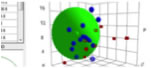
Grids:

An alternative way to create a set of solvents for the Sphere method is to use mixtures of pairs of solvents. The Grid option allows you to choose pairs of solvents, combined in a chosen number of Grid Steps and by clicking the Create button automatically generates the combinations and shows them as a plot in 3D graph.

 

 

Rather than use a full solvent name it is best to use an Abbreviated name. The HSP values can be put into the rows via the normal Ctrl-D from a master list and Ctrl-P into the appropriate rows.

 

The solvent choices can be loaded and saved as .grd files.

 

As a further option an AutoGrid can be created that is targeted to a particular area specified by the Target Zone inputs. By choosing Num. Experiments you intend to make and the Grid Steps this automatically works out the Num. Pairs to be created. The algorithm takes all the solvents currently in the Solvent Optimizer (as a convenient source of practical solvents) and examines each pair of solvents to see if they are useful for the Grid – i.e. they produce a scan line that crosses the target zone. If the Centered option is chosen then there is a bias towards scan lines that start and end on either side of the sphere.

 

It has proven very hard to decide on an optimum AutoGrid algorithm. But what is clear is that more important than the algorithm is the choice of solvents to be used! In other words, please put a lot of thought into the range of solvents within the Solvent Optimizer. It’s a good idea to carefully create a special Grid set which covers a good range of Grid space without too many duplicates. So there is no point in having both hexane and heptane in your solvent list because if a hexane:propylene carbonate scan line is good then it’s likely that the AutoGrid would also find that a heptane:propylene carbonate scan line would also be good – whereas it adds no real new data.

 

Please note that the grid is merely a way to do the boring work of setting up a reasonable solvent range – but users don’t have to use it blindly.

•   The user can easily delete points they don’t like and, if they want, add some pure solvents in key points. This is done in the main table, as usual.

•   The user has to check for miscibility and take into account MVol effects with, e.g. swelling.

•   The user can move the ranges based on their intuitions of where the test material will be.

•   It can be used to refine the radius if a solvent close to the middle is chosen as one of each pair.

  Please refer to e-Book grid page.