Abstract of HSPiP | Finding Hansen Sphere, Y-Fit
2012.Dec.21
We already have the HSP values of solvents. So we can plot those solvents in 3 dimensional (3D) space. Suppose, we have some solute (typically polymer) and set solvents' color blue that dissolve the solute, and set solvents' color red that do not dissolve the solute. If we view the colored solvents in 3D space, we will notice that the blue colored solvents are clustered and can fit into a Sphere. The program to get this sphere center and radius is a core routine of HSPiP. We have been developing many algorithms to determine these values and to use the visual information to understand solubility phenomena. Recently, we divided the Hydrogen bonding term (dH) into dHdo(donor) and dHac(Acceptor). And HSP became 4 Dimensional (4D). We need to design new Hansen Sphere viewer for viewing these alternative fits to see which best fits our data. For determination of Sphere Center and Radius, we present you HTML5-based software, "Y-Fit" as a Power Tool of HSPiP.
Browser support:
| Mac | Windows | Linux | |
| Chrome (ver. 23) | ◯ | ◯ | |
| FireFox (ver. 17) | ▲(Web Storge X) | ◯ | |
| Safari(ver. 6) | ◯(OSX, Lion+) | ? |
|
| Opera (ver. 12) | X (File API X) | ◯ | |
| IE (ver. 10) | - | ▲(Web Storge X) |
IE 6-8 does not support HTML5.
IE-9 does not support FileAPI so can not validate license file.
IE-10 has a problem in Local Storge and users need to validate every time.
Opera for Mac does not support FileAPI.
FireFox for Mac has a problem in Local Storge and users need to validate.
We strongly recommend Chrome browser.
Run the program
Please open index.html with an adequate HTML5 browser. (By clicking with right button and select open with application or drop index.html to alias of browser icon or, from HSPiP, clicking the PowerTools menu option) Then you will see the next startup screen. The language (English or Japanese), Button name and appearance are dependent on your browser. If you change size of browser window, the Canvas size is also change according to Window size.
Start up screen.
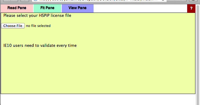
Validation
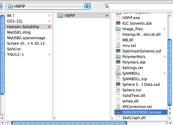
The first time you run a Power Tools, you need to register your HSPiP License File to the browser. Please click Choose File button (Button name and appearance are dependent on browser) and select your HSPiP License File, typically in c:\program files (x86)\Hansen-Solubility\HSPiP.
Once you open the License File, the browser stores the information locally and every Power Tools will run without verification. (IE10 does not handle local storage properly and users need to validate every time)
How to Use
After Validation, you will see the below window. (You may need to reload the browser)
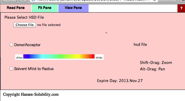
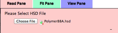
This Y-Fit program can read .hsd(Hansen Sphere Data) format datafiles. If you want to read the previous .ssd format file, please first open it with HSPiP and save it as hsd format. If you click Choose File button, you will be able to open files on your local disk. For practice purposes, find the files in your MyDocuments/HSPiP Data/Examples folder..
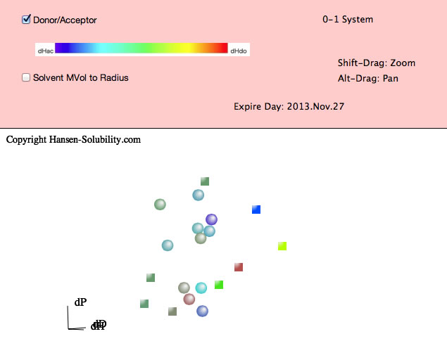
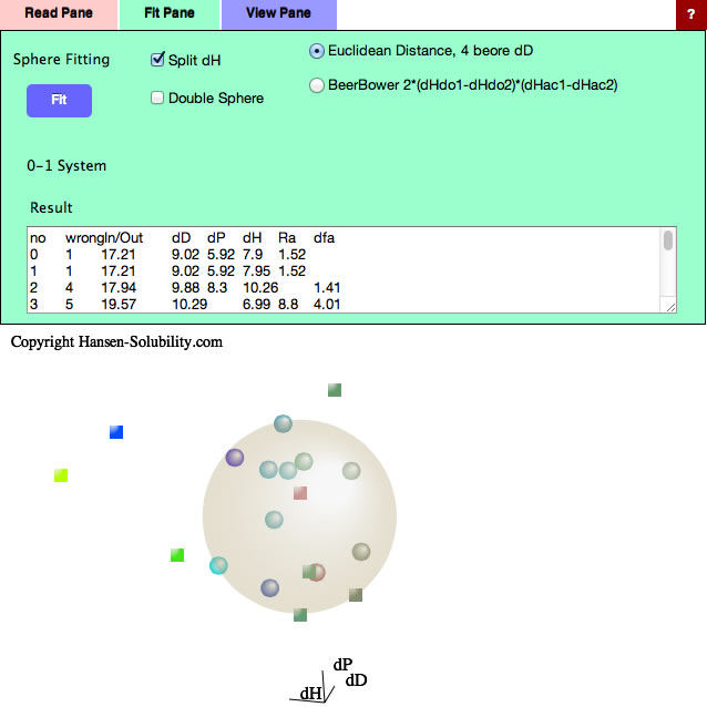
0-1 System
For example, please select Chapter4.hsd. Y-Fit reads the file and displays it as below. In this file, the Score is either 0 (outside sphere:color red) , 1(inside sphere: color blue) so the 0-1 system is assigned. If you drag inside the canvas, 3D Hansen space will rotate. If you click on a solvent, you will see the Hansen Solvent code (HCode) and solvent's name
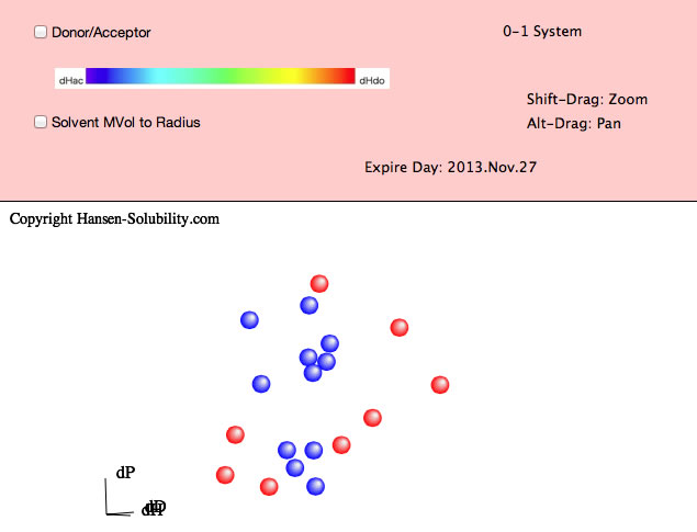
Shift-Drag zooms the view and Alt-Drag pans the view.
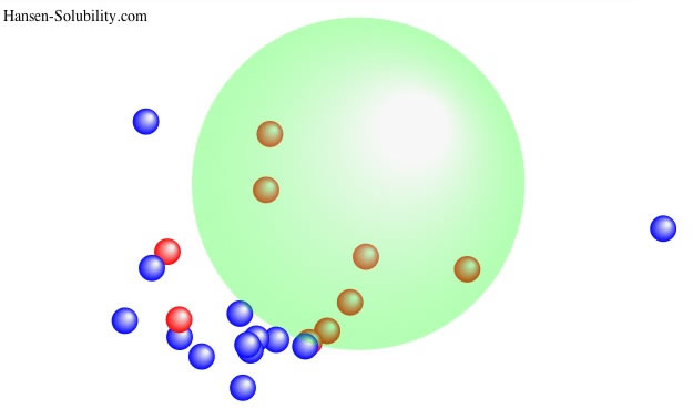
From HSPiP ver. 3.1, the dH(Hydrogen bonding term) was split to dHdo(Donor) and dHac(Acceptor) term. From the definition, dH²=dHdo²+dHac², so the position in Hansen Space is not changed. When the Donor/Acceptor option is selected, the color of the solvent means the ratio of of donor/acceptor. The blue color means donor nature solvents such as carboxylic acids. The red color means acceptor nature solvents such as amines. The green color means solvents have dual nature such as alcohols. The brightness of the color means the absolute dH value. For this appearance, we use color for ratio of of donor/acceptor and we can not distingush "inside"/"outside" solvents, so we adopt the HSPiP convention that "inside" are spheres and "outside" are cubes.
Then please click the Fit pane(Green tab), you will see the options that apply to the 0-1 system.
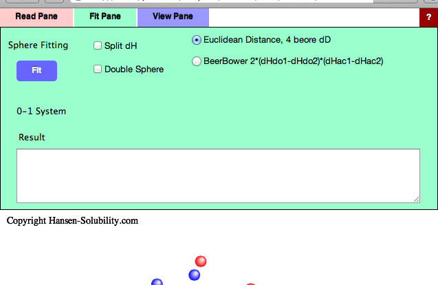
At first you need to assign HSP distance scheme. The normal HSP distance scheme is,
HSP distance= Sqrt(4.0*(dD1-dD2)² + (dP1-dP2)² +(dH1-dH2)²)
(Sqrt:Square root)
If you want to calculate 4 dimensional(4D) HSP distance (please check Split dH, the Canvas view will be changed), next scheme will be adapted.
4D HSP Dist.= Sqrt(4.0*(dD1-dD2)² + (dP1-dP2)² +(dHdo1-dHdo2)² +(dHac1-dHac2)²)
These are the most basic distance schemes in HSP.
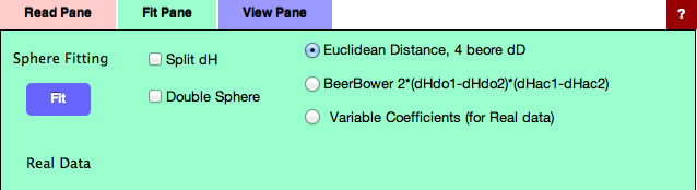
If you want to calculate 4D HSP distance, you can select Beerbower distance scheme.
Beerbower Dist.= Sqrt(4.0*(dD1-dD2)² + (dP1-dP2)² +2*(dHdo1-dHdo2)*(dHac1-dHac2))
If your target solute has large donor/acceptor interactions, the Beebower distance may work effectively, but solvents and solute distance viewed in 3D space become meaningless.
Click Fit with no options selected, you will see the View Pane.
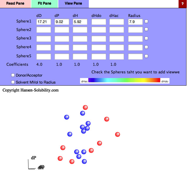
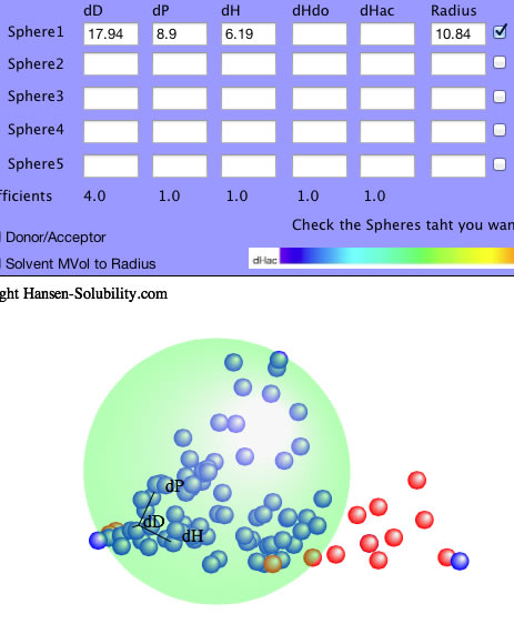
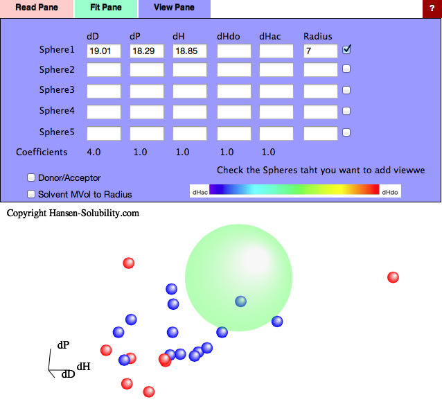
The program found [dD, dP, dH]=[17.21, 9.02, 5.92] and Radius=7.9 sphere. Check the right side checkbox, you will get the 3D view of solvents and Solute.
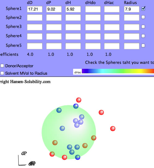
You can use the 4 other Sphere data boxes as you like. If you want to check a polymer's compatibility with the first solute, enter its HSP and radius and check the box to its right. If you want to check new solvents for this system, enter their values and view the solvent locations.
Go back to the Fit pane, all the results are listed in the textbox, so copy them and paste to Spread Sheet if you want to examine then further for analysis. The last column is a fitting quality parameter where smaller is better. You sometimes get a better fit quality but with a larger radius than the #1 value – it is up to you to decide which is more suitable for your system. Now check Split dH (The Canvas view will change).
(The color of the solute means nothing because dHdo/dHac of solute are not calculated yet.)
Then click the Fit button.
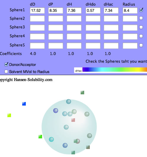
The dHdo=0.57, dHac=7.34 so this solute's nature is that of an Acceptor and the Sphere color becomes blue.
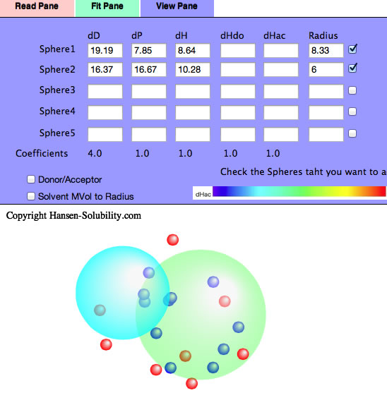
If you check the Double Sphere option, the program searches for 2 spheres that match Score=1 solvents located in either of the 2 spheres, and Score=0 solvents locate in neither of the 2 spheres.
The result of Double Sphere.
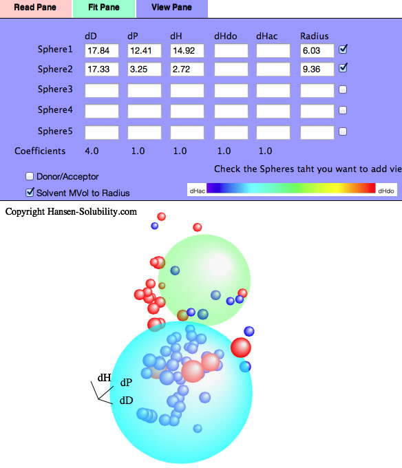
If you read Neoprene.hsd example and Fit, you will see several Score=0 solvents are locate inside Sphere(Wrong in). Check the Solvent MVol to Radius option, All such Wrong In solvents' molecular volume are very large. Click the solvent, then you will see the HCode and solvent name. You will find out those solvents are Phthalic esters. The Phthalic esters are used as plasticizer of polymer, and the plasticizer needs to dissolve in the polymer but must not bleed out. Then similar HSPs and large molecules are used for plasticizers. Plasticizer are poor solvents because they are too large and can not penetrate into polymers.
1-6 System
From the Read pane, please load the Polymer88A.hsd file.
For this file, the score is 1-6 system. Score=1 means the best solvents, and Score=6 are poor solvents. For this 1-6 system case, you need to set which scorer are assigned as inside. in the Fit pane, you will see the textfield and View button to press when you have changed the score. At first, solvents are colored by score.
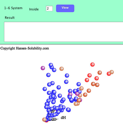
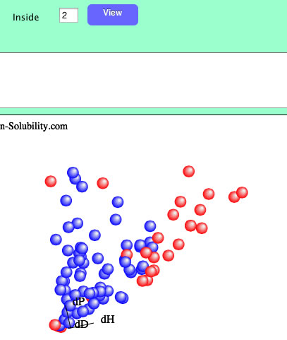
If you set inside as 2, Score 1-2 solvents are colored blue, and 3-6 solvents are colored red. You can change the definition of "inside" as many time as you like. Remember to confirm the effect by clicking the View button.
If you set 4 as inside.
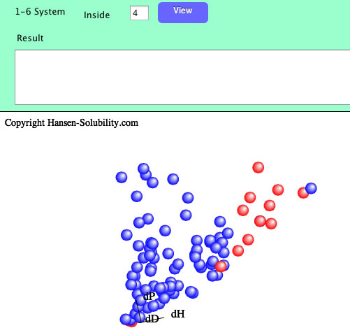
When you click the Fit button, Sphere will be searched with the textfield value.
All the options are same with 0-1 system after you set inside.
Score=1(complete dissolve)
Score=2(Swelling >100%)
Score=3(Swelling >70%),
Score=4(Swelling >30%)
Score=5(Swelling >10%)
Score=6(Swelling <=10%)
If you set Score like above, and changing inside 1 to 5. The Sphere center and radius will be different according to inside value. That will be helpful to understand your polymer solubility.
Real data
The HSP concept of solubility is generally a Qualitative analysis. We just select soluble (Score=1) or not soluble (Score=0). Even if we apply the 1-6 system, we only change the boundary of what we call soluble or nor soluble. In general, the nearer to the sphere center, the larger the solubility. But sometimes we encounter negative results.
For example, in the case of solubility of Paracetamol, suppose the solubility of solvent, log(g/Kg solv.)>2.0 set score=1 and otherwise score=0. That is 0-1 system and we can easily find Sphere like below.
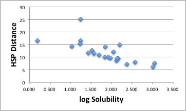
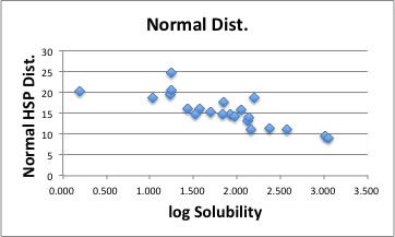
The center of Sphere becomes [17.65, 14.7, 17.49] and the radius is 9.45. There are 2 Wrong out solvents. If we plot this result as HSP distance vs log Solubility, you can find the correlation "The shorter HSP distance, the larger Solubility".
But look carefully!
If you want to try new solvents and you get HSP distance=15, can you estimate how much that solvents dissolve Parcetamol? How about HSP distance=8? The answer is “Yes” but the error margins are rather large..
From HSPiP ver 3.1, the Real data handling algorithm was added as a GA option. This algorithm searches the sphere center so the correlation factor between HSP distance and real solubility becomes maximal. Which solvents have the maximum extraction power? Which solvents make the reaction fastest? What will be the HPLC retention time of certain chemicals? This function is widely used.
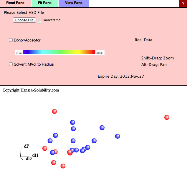
For example, if you read Paracetamol.hsd file, the data type is assigned Real Data. With our experience, you will get much better result if you take logarithm of solubility. And you'd better to set the data as "the shorter HSP distance, the more soluble". In HSPiP you have the option to invert the score value if the data are opposite - such as "amount left over when filtering the solution".
If you select Fit Pane, new option "Variable Coefficients" is added. (For real data you can not select Double Sphere)
Without options, just click the Fit button, you will get this result. For this real data handling, radius means nothing, so enter 7 for the purpose of visual effect.(If Radius=0, nothing appears)
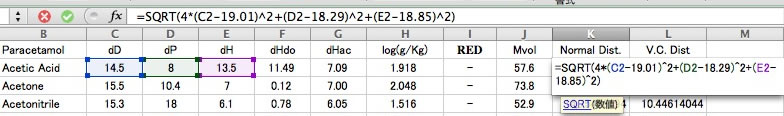
Normal distance calculation in HSP is
HSP Distance=sqrt(4.0*(dD1-dD2)² + (dP1-dP2)² + (dH1-dH2)²)
Let's browse this result with Spread sheet.
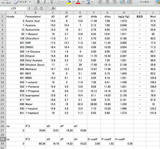
In an hsd file, dHdo and dHac is separated with / and this can not be handled as two numbers in the spreadsheet. You need to replace / with tab using a text editor.
And add the normal distance scheme.
You can plot the result.
The correlation is much better compair to 0-1 system. With this result, if the solvent's HSP is [19.01, 18.29, 18.85], the distance becomes 0 and the solubility is expected to be maximum.
Variable Coefficients Algorithm
If you calculate Paracetamol with Y-Predict, you will get [dD, dP, dH, dHdo, dHac]=[20.2, 13.3, 14.7, 11.6, 9.0]. Compare to the previous Fit result, [19.01, 18.29, 18.85], the dP difference is very large. Then we have the question whether the coefficients of HSP distance, (4,1,1,(1)) are adequate for quantitative analysis. So I made a new algorithm to Fit both HSP values and Coefficients value.
If you apply this Variable Coefficients option, The Sphere center become [18.16, 14.22, 18.23], and the Coefficients become [3.85, 1.52, 0.38].
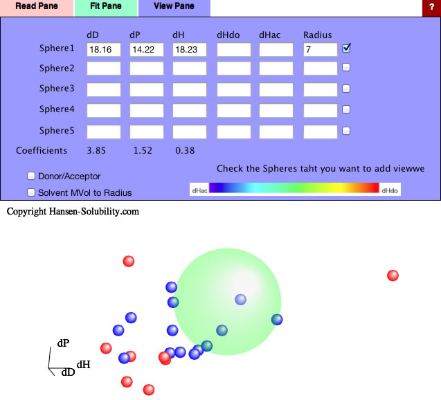
So the new HSP distance calculation scheme becomes as follow.
HSP distance=sqrt(3.85*(dD1-dD2)² + 1.52*(dP1-dP2)² + 0.38*(dH1-dH2)²)
The difference of dH will not work so much because the coefficients of dH is just 0.38, but the difference of dP works strongly because its coefficients is 1.52. We can understand solubility phenomena more accurately.

Let's browse the correlation of this result.
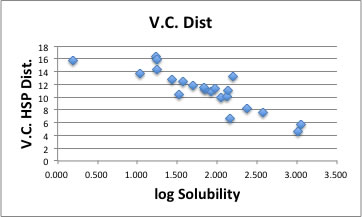
There are 2 exceptions but the correlation becomes so beautiful.
You can use the Split dH option.
You will obtain HSP[19.63, 14.06, 7.89,13.71], Coeffcients(4.38, 1.78, 0.24, 1.52).
This result is very close to the Y-Predict estimation
[dD, dP, dHdo, dHac]=[20.2, 13.3, 11.6, 9.0].
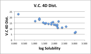
With this method, the coeffcients are dependent on solute. In other word, we fail to find universal HSP distance scheme for 4D Hansen (I mean a universal Donor/Acceptor interaction cross term).
I applied this Variable Coefficients option to many case, and in every case the Variable Coefficient 4D improves the correlation factor for quantitative analysis.