
2024.9.04
pirika.comで化学 > 化学全般 > 化学工学 > 復刻版:ASOGによる気液平衡推算法 > 第2章 ASOG法 > 2.3 実際のASOG法計算
2.3.1 1979年の例題の検証
1979年に講談社から出版された「ASOG法による気液平衡推算法」という書籍には例題として115系の例題が記載されている。その例題を実際に計算を行ってみよう。
グループ間相互作用パラメータln akl = mkl +nkl⁄Tのmkl,nklは,書籍に記載のパラメータを用いることにする(MN1979と呼ぶことにする)。例題は,圧力一定のデータが78系,温度一定のデータが37系ある。ポップアップ・メニューで系を選択すれば,必要なパラメータをデータベースから探し出し,ASOG法による推算値と実測値を比較する。
プログラムの使い方を説明しよう。
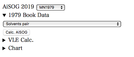
プログラムのページでは次のような初期画面になる。
セレクターという部品をクリックすると、次のようなメニューが表示される。
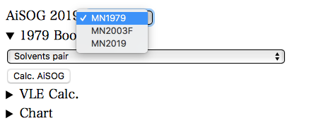
グルーブ間相互作用パラメータaklのバージョンを選択する。
(無償版ではMN2019は表示されない。ここでは、一番初期のMN1979を選択する)
次に溶媒ペアを選ぶ。
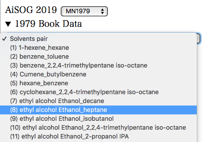
ここまでできれば、必要なパラメータは全て読み込まれている。
VLE Calc.の左側の三角形をクリックすると、折りたたまれていた部分が表示される。
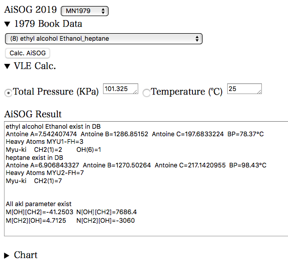
必要なパラメータはAiSOG Resultの部分に既に表示されている。
後は、圧力一定か、温度一定かをラジオボタンで選択し、Calc. AiSOGボタンを押す。1979 Book Dataの場合には、書籍に記載の圧力条件、温度条件が自動でセットされるので、Calc. AiSOGボタンを押すだけです。すると、条件に合わせた気液平衡が計算され結果がAiSOG Resultの部分に継ぎ足される。
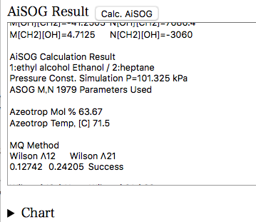
PCを使っているなら気液平衡のデータをコピーして表計算ソフトにペーストして利用するのでも良いだろう。簡単なチャートを描くプログラムも搭載してある。Chartの右三角をクリックして開く。チャートが表示されている。必要に応じて3種類のチャートをラジオボタンで選択する。
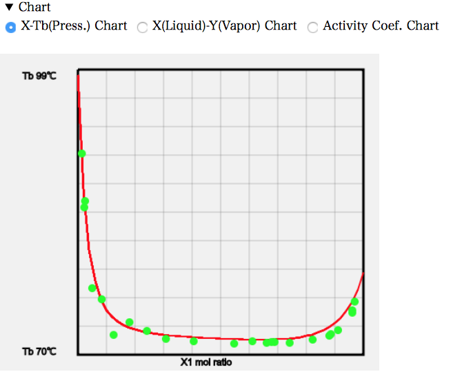
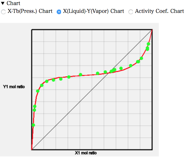
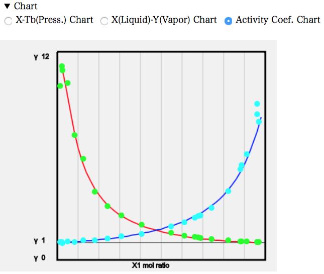
実験値のデータは緑色(水色)の丸で表示される。いろいろな系を選択して結果を眺めて見て欲しい。1979年にはこんな事ができていた。
こうしたことができるようになるとどんな応用があるだろうか?
例えば、冷蔵庫やエアコンに使われるフロン・ガスが大気に放出された場合のことを考えてみよう。紫外線で分解されたりしながら雨に溶けて地上に戻ってくる。流れ込んだ池や湖でどのような振る舞いをするのだろうか? 水との気液平衡がASOGで計算できると、蒸発しないで湖にとどまり続けるのか、大気に拡散していくのかわかる。
ヘンリーの法則(Henry’s law)という法則がある。揮発性の溶質を微量含む溶液があった場合には、溶質の分圧は溶液中の濃度に比例する。その比例定数のことをヘンリー定数と呼ぶ。ヘンリー定数が大きい溶質は、濃度以上に気相に飛び出したがっている事になる。
例えば、水と、いろいろなエステル化合物との気液平衡を推算して、その時の無限希釈活量係数(Magules A)と、このヘンリー定数の文献値を比べてみる。
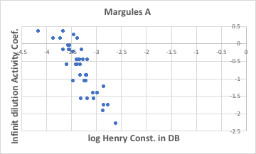
文献値が全くない場合には、このような方法でヘンリー定数を推算するということがよく行われている。環境関連の研究には無くてはならないツールと言える。
今回作成したシミュレータでは直接計算できるのは、活量係数だけになる。
しかし、こうした活量係数は使い方によっては非常に有用な情報を与えてくれる。
Copyright pirika.com since 1999-
Mail: yamahiroXpirika.com (Xを@に置き換えてください)
メールの件名は[pirika]で始めてください。