Chapter 10               Insoluble solubility parameters (HSP for Pigment Surfaces)

A lot of the colours we see around us come from pigments. By definition these are insoluble, so it seems to make no sense to worry about their “solubility parameters”. Yet the HSP approach has proved immensely valuable – giving lots of practical insight for comparatively little work. In this chapter we’ll stay mostly in black, with the various forms of insoluble carbon. Yet the principles apply to pigments of any hue.

It seems an admission of defeat to introduce the concept of a pigment being “happy” in a solvent. How can such a term apply to something as scientific as HSP? Let’s turn the question around. As a scientist, you can shake up a sample of, say, carbon black in a solvent and know that the pigment is happy or unhappy in that solvent. For example, a happy carbon black will go into dispersion in a solvent with a mere shake of the test tube. An unhappy carbon black will simply sit as a lump in the bottom of the test tube no matter how much you attack it with high energy ultrasound. If you use a range of solvents covering HSP space you can form a judgement of happy/unhappy and put those data into HSPiP and calculate the HSP of the carbon.

For those who want to be more sophisticated, you can score the happiness in more objective ways. For example you can measure the sedimentation rate and assign numbers on the basis that faster sedimenting pigments have poorer solvent interaction than slower ones. However, note that Ch.7 of the Handbook introduced the concept of RST – Relative Sedimentation Time – to help correct for differences in sedimentation due to density/viscosity:

RST=t_s(ρ_p- ρ_s)/ η

where t_s is the actual sedimentation time, ρ_p and ρ_s are the densities of the particles and solvent and η is the viscosity. The RST values, rather than the raw t_s values should then be used to decide between “good” and “bad” solvents.

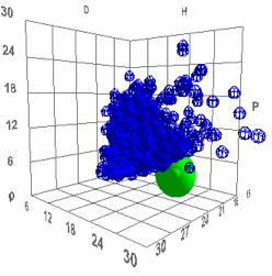
Either way, you will find yourself with a plot such as the following:

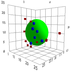
Figure 1‑1 Using file CarbonBlackLow

If you try a different type of carbon black you find a very different result:

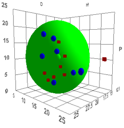
Figure 1‑2 Using file CarbonBlackHi

These two simple experiments reveal a profound difference between two pigments both labelled “carbon black”.

	δD	δP	δH	R
CarbonLow	16.2	10.2	7.3	8.3
CarbonHi	20.5	11.0	12.1	10.8

Table 1‑1 Comparison of parameters for CarbonLow and CarbonHi

Indeed, there are many different types of carbon black with very different surfaces and therefore very different abilities to interact with solvent or polymer binder. If you don’t have the HSP, how can you rationally optimise your carbon black formulation?

If your binder and pigment have identical HSP then you have perfect compatibility. But what do you do when you have a coating containing pigment, binder and solvent? It seems obvious that your solvent should also have the same HSP. But this would mean that the binder/solvent interactions were so strong that the binder/pigment interactions could be overwhelmed. If the binder has HSP somewhere between the solvent and the pigment, and if the solvent is on the boundary of the binder then parts of the binder will tend to associate strongly with the pigment, probably leaving its solvent-compatible parts on the outside and thereby giving very good solvent compatibility for the whole system, whilst ensuring that the binder is nicely locked on to the pigment when the solvent evaporates.

Just pause to think on that paragraph. All you need in order to come up with a good starting point for a practical pigment dispersion are the HSP of pigment and binder. With help from the program you can rapidly identify a solvent that is on the outer rim of the binder sphere, with the pigment still further away.

Let’s try it with PMMA and the CarbonBlackHi. Load a typical list of solvents (such as FriendlySolvents), select PMMA in the Polymers form, make sure you’ve selected PolymerR so that RED numbers are calculated on the basis of PMMA’s radius, and click the Solvents button. When you look for solvents with a RED number ~1 (i.e. on the border), MIBK looks a good fit.

	δD	δP	δH	R
PMMA	18.6	10.5	7.5	8.6
CarbonHi	20.5	11.0	13.2	11.1
MIBK	15.3	6.1	4.1	RED=1

Table 1‑2 Finding a borderline solvent

If you wanted a good place to start to generate a good formulation using PMMA and this carbon black, then MIBK would be a good place to start.

If you were using the CarbonBlackLow you would, of course, choose a very different solvent.

As this is a chapter about the truly insoluble, we introduce a pleasing digression. We came across a wonderful YouTube video http://www.youtube.com/watch?v=jQdCRARzOv8

which shows how to determine the solubility parameter of glass. You simply find which liquids completely wet the glass (“Good”) and those which don’t (“Bad”) and run the Sphere correlation. We are grateful to Dr Darren L Williams of Sam Houston State University, Texas for permission to reproduce his data here.

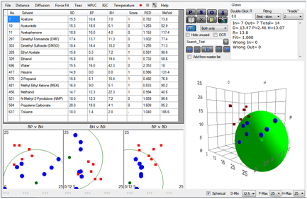
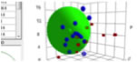
Figure 1‑3 The HSP of glass

As you can see, glass is estimated to be [13.5, 2.5, 13.1]. It will be very interesting to see if Dr Williams’ technique can be extended to other surfaces and add insights beyond the traditional surface energy calculations. As surface energies are often broken down into sub-components such as Dipolar, Polar, Lewis Acid/Base it would seem an interesting research project to see if the HSP breakdown into δD, δP, δH proves to be fruitful in understanding surfaces. It is worth noting how unusual this HSP set is. By using the entire Sphere Solvent Data set and putting the glass values into the Polymer table and clicking the Solvents button, the glass sphere is outside the entire solvent range. It will be interesting to know if this is an artefact of the fit or a real insight into the glass surface:

 

Figure 1 ‑ 4 The glass sphere plotted in the context of the entire Sphere Solvent Data set, showing how unusual it is

This is our first venture out of the “solubility” comfort zone of HSP. Let’s carry on to see another area where the last thing you are interested in is polymer solubility.

 

E-Book contents | HSP User's Forum