Chapter 2, The Sphere (The Preferred Method of Visualizing)

If 2 parameters were good enough to work, then life would be very easy and HSP would be used much more frequently. You could plot everything on a nice X-Y graph.

The problem with HSP is that they need to be plotted in 3D. With modern software this isn’t so hard. But for papers and books it’s more usual to use 2D plots and this creates an interesting problem.

Most people associate HSP plots with δP v δH graphs, Polar versus Hydrogen bonding. If you have to have just one plot, then this is the most important. But this tends to diminish the significance of Dispersion, which is unfortunate. As 3D graphs are hard to understand when shown statically in a book, we will sometimes have to give you sets of 3 graphs, P v H, H v D, P v D. This is a bit cumbersome, but it’s better than leading you astray with just the P v H plot. Because you get the software with this book, we generally supply just the 3D plot and urge you to look at each example live as it is a richer interactive experience.

P v H means H is plotted along the X axis and P along the Y axis and similarly for H v D and P v D..

But first let’s see what the Sphere can teach us.

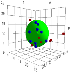
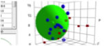
Figure 0‑1 Using file Chapter2

Let’s orient ourselves. The graph shows the P-axis going vertically from 0-25. The H-axis also goes from 0-25 from left-to-middle right. The D-axis goes from 12.5-25 from right-to-middle left. In the program you can orient the plot any way you like, but in the book we will always keep this orientation.

There is a large green sphere. In the exact centre is a green dot. This shows the position of a particular polymer with values D=18.5, P=9.9, H=7.9. There is a set of blue dots. These are all inside the sphere (though that is not obvious from the static view on the page). They are located at the HSP of solvents which dissolve this polymer. The red cubes show the solvents which do not dissolve this polymer.

The program has taken the will/won’t dissolve data of each solvent and calculated the sphere which includes all the good solvents (defined in HSPiP as “Inside” the Sphere) and excludes all the bad solvents. If the sphere were any smaller then it would exclude some of the good solvents and if it were bigger it would include some of the bad solvents. And of course if the calculated centre of the sphere were in any other position the sphere would exclude/include good/bad solvents.

In this example, 16 solvents have been used, 9 of them are good and 7 of them are bad. Some of the solvents used for the test are definitely not ones you would want to use if you wanted to dissolve lots of this polymer. The list includes chlorobenzene and nitrobenzene. We will see later on why we include unpleasant solvents in the tests.

If you wanted to find a good solvent to dissolve this particular polymer you would find that there isn’t any close match amongst reasonably safe solvents. However, a 77:23 mix of 1,3-Dioxolane and Ethylene carbonate is a good match.

Here’s the first reason you need Sphere. This reason is based on the centre of the sphere, which shows you the optimum HSP for good solvency. How likely is it that you would have come up with this particular 77:23 mix by chance? It’s highly unlikely. In all probability you’d have very little idea of what an optimum could/should look like and you would be even more unlikely to come up with that near-ideal mixture.

Incidentally, if you used a classic 2D HSP plot you would conclude that acetone is near-perfect match. In H-P space it is perfect but the D value is way off.

The second reason is based on the radius of the sphere. There are plenty of reasons why you wouldn’t want to use that 77:23 mix, which is optimal only for thermodynamic solvency. You might want to reduce cost or meet some environmental regulations. So you need to find a solvent mix which is “good enough”. What is the definition of “good enough”? It’s simple. If a solvent blend is inside the sphere then it’s likely to dissolve the polymer and the closer it is to the centre, the better it is.

So you can now play around with solvent blends in a rational manner. Simply calculate their weighted average HSP and check how close they are to the centre of the sphere. If you want to be really sophisticated (and in a later chapter we show how to use the HSPiP Solvent Optimizer to do this), you can do an optimisation using the HSP distance from the centre as one parameter (bigger is worse, and outside the radius is scored as infinitely bad) along with, say, cost and environmental impact as the other parameters. How you choose to weight these three different parameters only you can say. But without knowing both the centre and radius of this polymer you would not know where to start.

To do that optimisation you need to know “the HSP distance from the centre”. How is this calculated? You already know the answer:

Equ. 0‑1 Distance² =4 (δD_A-δD_B)² + (δP_A-δP_B)² + (δH_A-δH_B)²

And that’s all you really need to know about HSP and the Sphere!

But because the term is widely used and is a useful shortcut, let’s give you one more concept.

The RED number is the Relative Energy Difference and is simply the ratio of the distance of your solvent (blend) to the radius of the Sphere. A perfect solvent has a RED of 0. A solvent just on the surface of the Sphere has a RED of 1. It is a useful shorthand that gives quick insights into what’s going on. Relative REDs are useful. If you have a solvent of RED 0.2 and another of 0.4 you know (a) that neither is perfect and (b) that the first one is better.

Let’s see how the RED number can help you avoid a simple mistake. We promised that we’d show you some of the 2D plots. Here they are for this example:

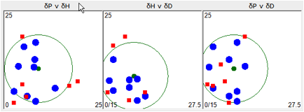
Figure 0‑2 Using file Chapter2

In the program, as you move the mouse over each plot you get a read-out of each solvent’s name and HSP. Note how misleading these plots are. Two “red” solvents are inside the P v H plot which is what most look at. If you relied only on that plot you would be easily confused. For example the red square on top of the blue dot at 7 o’clock in the P v H plot are diethyl ether [14.5, 2.9, 5.1] which is a non-solvent and trichloroethylene [18, 3.1, 5.3] which is a solvent. Their RED numbers are 1.33 and 0.89 respectively which indicates that diethyl ether is significantly outside the sphere. In this case it is obvious that the low D of ether (14.5) makes it highly unsuitable for a polymer with a D of 18.5. The trichloroethylene’s D value of 18 explains why its RED is so much lower.

As we will find in the chapters which follow, the beauty of Sphere is that it captures the essence of a huge variety of different phenomena. Armed just with the HSP of solvents (or solvent blends) and the HSP and radii of polymers we can make reliable predictions that work both in the domain of pure science and in the world of industrial applications. Although HSP have their limitations, it is hard to find an alternative approach that combines thermodynamic soundness with practical insight.

Let’s first see how HSP can be applied to a basic issue – cleaning up an ink or paint by dissolving the polymers which hold the ink or paint together.

Note For those who like triangular graphs we’ve added the Teas plot, named after Jean Teas its inventor. It simply plots δD/(δD+δP+δH) along one axis against δP/(δD+δP+δH) on the next and δH/(δD+δP+δH) on the third. Although this is a neat way to condense 3D data into 2D, there is no scientific significance to the plotted values! A perfect Sphere with all “good” inside and all “bad” outside can look a muddle in the Teas plot. However, some people find it visually useful. As a visual aid, the computed centre and radius are plotted using their own (δD+δP+δH) value along with the “bounding circle” and its centre. Again these have no great scientific significance. When you move your mouse over the Teas plot you get either the % δD, %δP, %δH or if you are near a solvent, the actual δD, δP, δH and the solvent name.

 

 

E-Book contents | HSP User's Forum