In earlier editions of HSPiP we took it for granted that the explanation in the previous chapter was sufficient to help users calculate their first solubility Sphere. But we found that users were very unsure of themselves and we often had to email advice to them. Thinking back, one of us (Abbott) remembers how nervous he was with his first Sphere, so the following practical guide reflects his memories of his first Sphere, backed up by the experience of measuring many different Spheres over 40 years by Hansen.

Let’s start with a typical example. You want to dissolve a polymer for some sort of processing such as coating. You have severe restrictions on cost, health & safety or environmental impact so finding a good solvent blend is very hard. If, instead, you are interested in dispersing a pigment or nanoparticle, the discussion below is identical, just substitute “pigment” or “nanoparticle” for “polymer”.

Our task is to define the HSP of the polymer. A solvent (blend) that is close to that HSP will be a good solvent. Here’s how to do it.

Get about 20 glass vials. Put a small sample of the polymer into each of the vials. Now add a small amount (say 5ml) of a different solvent to each of the vials. Which solvents should you use? Well, the following list is a pretty good mixture of relatively common and relatively safe solvents. It’s included as Test Solvents.hsd with the package and you can easily add/remove solvents to suit your needs.

 

Solvent	D	P	H
1.4-DIOXANE	19	1.8	7.4
1-BUTANOL	16	5.7	15.8
2-PHENOXY ETHANOL	17.8	5.7	14.3
ACETONE	15.5	10.4	7
ACETONITRILE	15.3	18	6.1
CHLOROFORM	17.8	3.1	5.7
CYCLOHEXANE	16.8	0	0.2
CYCLOHEXANOL	17.4	4.1	13.5
DBE	16.2	4.7	8.4
DIACETONE ALCOHOL	15.8	8.2	10.8
DIETHYLENE GLYCOL	16.6	12	20.7
DIMETHYL FORMAMIDE	17.4	13.7	11.3
DIMETHYL SULFOXIDE	18.4	16.4	10.2
DIPROPYLENE GLYCOL	16.5	10.6	17.7
ETHANOL 99.9%	15.8	8.8	19.4
ETHYL ACETATE	15.8	5.3	7.2
GAMMA BUTYROLACTONE	19	16.6	7.4
HEXANE	14.9	0	0
MEK	16	9	5.1
METHANOL	15.1	12.3	22.3
METHYL ISOBUTYL KETONE	15.3	6.1	4.1
METHYLENE DICHLORIDE	18.2	6.3	6.1
n-BUTYL ACETATE	15.8	3.7	6.3
N-METHYL PYRROLIDONE	18	12.3	7.2
PM	15.6	6.3	11.6
PMA	15.6	5.6	9.8
PROPYLENE CARBONATE	20	18	4.1
TCE TETRACHLOROETHYLENE	18	5	0
TETRAHYDROFURAN	16.8	5.7	8
TOLUENE	18	1.4	2

 

But if you don’t have all of them, no matter. And if you have some others that’s fine. Just don’t have too many of the same thing. It probably doesn’t help to have methanol, ethanol, propanol and butanol or pentane, hexane, heptanes and octane. Just ethanol and hexane will be good enough.

Now you need to find out in which solvents the polymer is soluble. Here you have to make a decision. You can, for example, just hand shake each sample and then see which ones give clear solutions and which ones don’t. But often you find that such a test is useless as even good solvents might take some time to dissolve your polymer. So you might decide to put all the vials into an ultrasonic bath for 10 minutes then inspect each vial as soon as it comes out of the bath. But often you find that everything gets dispersed by the ultrasonics so that everything looks to be “soluble”. So you might decide to check after  the samples have sat for 10 minutes at room temperature. And maybe the polymer doesn’t “dissolve” in any of the solvents (perhaps you had too much polymer or too little solvent) but you can still see that the polymer is highly swollen in some solvents and completely unswollen in others so you can use that as your criterion for “good” and “bad” solvents. For some polymers you might even have to wait for days to distinguish “good” and “bad”.

Don’t despair if the previous paragraph is too vague for you. You are a scientist and you probably already have a good intuition about the general solubility properties of your polymer, so you can make a good decision about what treatment to adopt and whether you judge by dissolution or by swelling.

One word of advice. Because the effects of temperature on solubility can be quite complex, stick with room temperature tests if possible – at least till you have gained some experience in the whole process.

And if you aren’t interested in polymers but in, say, pigments, the above description applies to you too. Just find a set of conditions where your pigment is obviously “happy” in some solvents (e.g. nicely and permanently dispersed) and “unhappy” (e.g. sitting as a lump at the bottom of the vial) in others. Be careful to check if any pigment is stuck on the side of glass containers.

If you are lucky (or already have a good intuition) after a moderate effort you now have a list of good and bad solvents. If your system is entirely new then you might spend a day finding the appropriate test conditions, sometimes getting sidetracked when a “clear” solution is in reality a blob of polymer stuck under the cap of the vial. But once you have your list of good and bad solvents then the Sphere calculation does the rest.

With all the scores entered, 1 for good and 0 for bad, you click the Calculate button and you get two vital bits of data, both of which are important. The first is the HSP of the polymer. That’s defined as the centre of the Sphere. Any solvent close to that centre will be excellent for that polymer. But how close is “close”? That’s why you need the second bit of data which is the radius of the Sphere. You’ll remember that RED number is the ratio of the distance of a solvent from the centre of the Sphere, divided by the radius of the Sphere. If your polymer gives a small radius, say, 4, then a solvent with a distance of 4 is just on the boundary – the RED is 4/4=1. A solvent with a distance of 8 is therefore a bad solvent, with a RED of 8/4=2. But if your polymer is more forgiving, then the radius might well be 8. So the solvent with distance 4 now has a RED of 4/8=0.5 which means that it’s likely to be pretty good. The solvent with the distance of 8 now has a RED of 8/8=1 so is borderline.

The previous paragraph is so important that you need to read it again till you’re 100% clear. Both the centre and the radius of the Sphere are vital for you to know. Later on, when you understand the Polymers form in HSPiP you’ll find some tricks for working out which solvents (usually from a list that is different from the one you used to determine the Sphere) are good or bad. By adding your polymer (both HSP and Radius) to the Polymers form with one click you’ll be able to sort your solvent list in order of RED – with the low REDs being the good solvents.

Here’s an example (included in HSPiP) where the Sphere comes out best matched to chloroform. You can instantly tell that it’s the best match because the solvents are sorted by their RED numbers and chloroform has the smallest RED. In later chapters we will see how you can find a solvent blend that would be a close match to chloroform and the centre of the Sphere, but without the (probably) unacceptable use of chlorinated solvents.

 

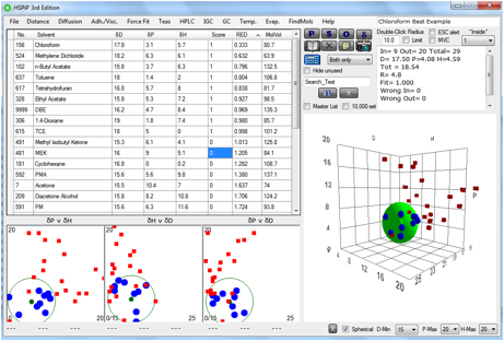
Figure 0‑1 A typical first Sphere test using a typical, sensible range of solvents

Bad Spheres

There are two types of bad Spheres that come out of such experiments.

1 The first is a Sphere with (approximately) the same values each time you click the Calculate button, but with an appallingly bad fit – with many good solvents outside and bad solvents inside. In general there are three possible reasons for this

·      You’ve made some misinterpretations of your data. It’s quite common, for example, to go back to recheck a “good” result which doesn’t fit the Sphere, only to find that the polymer is stuck underneath the lid of the test-tube rather than, as we thought, being nicely dissolved. When you correctly class this as “bad” the Sphere fit greatly improves

·      HSP just don’t apply to your system. This is possible, but unusual. Pigments with highly charged surfaces may fall into this category

·      Your test material is impure. In fact we have often proved that materials are impure by finding bad HSP Spheres and alerting researchers to look out for (and find) impurities

·      Your material has a split personality – e.g. a 1:1 block copolymer made from hydrophilic and hydrophobic parts. In principle we could force HSPiP to generate two Spheres, but we’ve never been convinced of the value of this. But see v3.1!

2 The second problem shows up as a Sphere which appears in a different place each time you click the Calculate button. This is simply a case where you don’t have enough good/bad solvents surrounding the centre of the Sphere to create an unambiguous best fit. For example, if the real δD is ≥19, the chances are that you’ve used very few solvents up in this range. There is no way to know if the real δD is 19 or 20 or 21 because there are no δD=21 solvents giving you a “good” or “bad” result. The only way you can pin down the real Sphere is to work out (it should be obvious looking at the 3D plot and the 3 2D plots) where you are lacking data.  Then simply find a few relevant solvents and do the tests. We mentioned earlier that sometimes you have to use nasty solvents in tests. You may well be forced to use such solvents to get data from a relevant region. As long as you can handle the solvent safely for the test, it doesn’t matter that it too nasty to be used in a real application. Remember that you don’t have to re-do any of your previous tests. You simply add the new data to your list and click the Calculate button.

This still doesn’t explain why the “best fit” moves around so alarmingly. This is for two reasons – one mathematical, one philosophical

HSP 3D space is quite complex. If you could test each point in that space to see if it’s the best (or least bad) fit to the data you would find in the case of really good data sets that there is a clear, deep well down into which any good fitting algorithm would quickly fall, finding the same result each time it started, from wherever it started. With under-specified datasets, there are no such deep wells and it’s very easy to fall into a shallow well, thinking that it’s the best. So the “best” fit depends on your starting assumptions. This is typical mathematical behaviour.

Philosophically we could make ourselves look good by always leading you to the same false fit, however often you clicked the Calculate button. But we deliberately want you to see when the fit is poor. The fact that you see a different “best” fit each time is telling you clearly that the dataset is under-specified and that you need to gather more data points if you really want to know the centre and radius of the Sphere. Each time you click the Calculate button, the fitting algorithm starts from a totally different part of HSP space and therefore, in the case of under-specified data, is likely to end up in a different “best” fit each time.

However, for the 3^rd Edition we’ve been able to find a better way to search the whole 3D space and the “jumping around” problem has been much reduced.

Changing the fitting algorithm

The “classic” Hansen fitting algorithm has been used successfully for over 40 years. It systematically explores the whole of HSP space and weighs the errors of good-out and bad-in depending on how badly out(in) a solvent actually is. This makes a lot of sense. But one very wrong point can exert a disproportionate effect over the fit. We’ve therefore provided the option of a totally different way of identifying and finding a best fit. The GA (Genetic Algorithm) attempts to find the least wrong solvents within the smallest possible radius. The search is via the genetic approach using “genes” that create the fit and selecting better genes throughout the generations. Not surprisingly, the two approaches often reach a near-identical result and the classic approach tends to be faster than the GA algorithm in these cases. But in other situations (e.g. with odd outliers) the GA result seems more intuitively satisfactory than the classic approach. You, as a scientist, can reach your own judgement for your own cases.

Changing the definition of “good”

A lot of people are worried about the flexible definition of “good”. It doesn’t sound precise enough to be good science. So as an exercise, take the above sample file and deliberately set two of the solvents near the edge of the Sphere (RED ≥0.98) to “bad”. This could happen, for example, if a colleague looked at your test tubes and said “I think you are being too generous in your evaluations. I don’t think that dioxane and TCE are good – they should be classed as bad”. When you calculate the Sphere you get new values [17.10, 3.07, 5.10, 4.10].

The changes in this case are typical of what you find in real-world examples. The centre of the Sphere does not change all that much, but the radius changes, in this case by quite a lot (from ~8 to ~4). This is an important result. The key “truth” about this polymer reside in the HSP. These don’t change much when you change your definition of borderline good/bad. The radius is an important part of the HSP characterisation of a polymer, but it must be variable – for example a lower molecular weight version of the same polymer will be more soluble and have a larger radius.

Please do try this playing around with the data. If you eliminate more and more solvents then, of course, the Sphere will start to move around more. You can’t be too careless about the definition of good. And when you are down to just a few good solvents, the data become statistically less satisfactory. If you find yourself in this situation you have no other choice than to find a few more solvents in the critical region and testing those for good/bad. If you find one or two more good solvents then your confidence in the HSP of the polymer will improve.

Rational improvement

One user of HSPiP asked if we could add a feature to help rationally improve the quality of the fit. What he wanted was an automatic scan of the 3D fit to identify “diversity voids”, i.e. areas in 3D space where there is no relevant data. For HSP, “relevant” means ‘close to the edge of the Sphere and in an area where there are no other solvents’. Why is this important? If you test extra solvents that are either near the centre of the Sphere or near another solvent or are far outside the Sphere, you get very little extra information. But if you find a solvent near the edge, and in a direction where there are no other solvents then this one extra data point could be crucial for defining the edge.

We’ve found a relatively simple way to implement this process. A file called SphereCheckMaster.hsd contains a list of 80+ solvents that fill a good part of 3D space. These solvents are a subset of the original Hansen 88 solvents so their values are well-validated. When the Sphere fit has taken place, the software scans each of the solvents to see if it is near the edge of the Sphere (i.e. 0.9<RED<1.1) and if it is whether it is far enough away from the other solvents used for the fitting. If both those tests are passed then the solvent is shown in the plots in orange and added to the table of solvents. As an intelligent user you can then make the judgement as to whether any or all of those solvents would really be worth testing. If you are happy with “good enough” then you may not even want to do this Sphere Radius Check (SRC). If you do the check you might disagree with the program’s judgement on some of the solvents but might agree that one or two of the solvents might be worth doing. You might then find that one of these solvents is unacceptable in your lab. At that point you can highlight that solvent and go into Solvent Optimizer to find if there is a blend of nicer solvents that could be used instead.

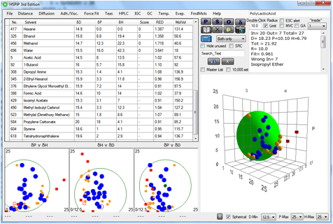
Figure 0‑2 12 solvents (in orange) suggested by the SRC check.

In summary, the SRC is a tool that you are free to use to help you decide on whether it’s worth doing more experiments. It’s certainly not a perfect tool (there are probably more sophisticated algorithms that could be used) but we find it helpful so we hope that you will too.

Using numeric data for greater accuracy

If you can go to the trouble of measuring actual solubility of the polymer rather than Yes/No solubility then you have richer data and the chance to get a more accurate fit. The Data fit method in HSPiP will, therefore, provide a more accurate value, especially if fewer solvents are used. Clearly there is a trade-off: there is more work required to measure the solubilities, but less solvents (if chosen carefully) are required.

An alternative numeric approach uses measurements of the intrinsic viscosities of the polymer in the solvents. The idea behind this is that the better the solvent, the higher the viscosity (because the polymer opens out more). The equations for fitting to intrinsic viscosity data are simple as discussed in, for example, Farhad Gharagheizi, Mahmood Torabi Angajia, A New Improved Method for Estimating Hansen Solubility Parameters of Polymers, Journal of Macromolecular Science, Part B: Physics, 45:285–290, 2006. If HSPiP users would like us to implement those equations we would be happy to do so.

Remember, however, that the use of limited numbers of solvents comes with the danger of not encompassing sufficient of HSP space. Fitting algorithms can always find an optimum, but if there are no solubility data in important parts of HSP space then these optima will be false. Many polymers have one or more of the HSP higher than any potential test solvent. Simple averaging the HSP of the test solvents, weighted in any way, cannot lead to the correct answer. The sphere fitting process is required. The intrinsic viscosity inherently limits a study to those solvents that do dissolve the solute. There are in essence no “bad” solvents for measurement of the intrinsic viscosity, but ranking the intrinsic viscosity into the standard 1-6 ratings, possibly with a 0 for those solvents known not to dissolve the solute, will allow an analysis in the usual way.

 

E-Book contents | HSP User's Forum