Chapter 31, Predictions (Many Physical Properties are Correlated with HSP)

The more powerful the theory, the better its ability to make predictions. This chapter shows that HSP can provide the basis for some very powerful predictions in important areas. The HSPiP software implements each of the predictions in turn: HSE, Azeotropes/Vapour pressures, Solubilities.

HSE

The HSE modeller captures in one place all the capabilities we have for making rational choices about chemicals in terms of Health, Safety and Environment. It lets you enter the SMILES for two chemicals and then lets you compare a large set of important properties. A typical example is “read across” for REACH and other chemical safety systems. If you know that a particular chemical is safe or unsafe then a rational starting point for judging the safety properties of an un-tested material is to “read across” from this chemical to a similar one. But how similar is similar? Only you as a scientist can judge, but in the HSE comparison you can compare estimates of

·      Phase change properties – melting point, boiling point, vapour pressure

·      Solubility properties – solubility in water, Octanol/Water partition coefficient, Soil/Water partition coefficient, BCF (Bio Concentration Factor) for Fish oil

·      VOC properties – RER, vapour pressure, flash point, OH radical reactivity, Carter MIR

·      Other properties – Heavy Atom Count, Density, Molecular Weight, Molar Volume

·      Numerical comparison – HSP distance, “Functional Group distance”

The functional group distance is an estimate based on the (dis)similarity of the functional groups derived from the Y-MB analysis. If, for example, the two molecules both of FG#27 (primary alcohol) then their distance is lower than if one has FG#27 and the other has FG#38 (primary amine) which in turn is larger than between FG#27 and FG#28 (secondary alcohol). The methodology takes into account the different molecular sizes and the numbers of functional groups. Clearly a molecule with many functional groups must be quite distant from one with just a few, even if those few match groups in the larger molecule. To ensure that differences aren’t too exaggerated, although butanol has 4 carbons and methanol has only 1, each molecule is shown as having just two functional groups, and the distance between methyl and butyl is not all that large. This calculation is different from one which would count similar methyl and alcohol groups in both molecules but would have two un-matched CH₂ groups in the butanol.

A note on LogP=LogKow=Octanol/Water partition coefficient

LogP is often seen as a highly important parameter. Although it is important we think that it is very much misused. In our view, HSP are very often much more insightful than LogP. The main reasons we are sceptical about LogP are:

·      It is a ratio which can hide important details. A LogP of 0 (i.e. P=1) could have solubilities of 100/100 or 0.001/0.001. Chemically the former (high solubility) is likely to be very different from the latter (low solubility) even though the ratio is the same.

·      Chemicals in biological environments don’t have a choice between a “water” environment and an “octanol” environment. A typical lipid environment might be much closer to [16, 3, 3] than octanol’s [16, 5, 12] and as we showed in another chapter, a lot of key biological entities such as skin or DNA binding sites are closer to [17, 10, 10] than to octanol. LogP is far too restricted to be able to give a reliable guide to where a chemical might be going.

But as a service to HSPiP users we felt it was important to provide the best-possible predictor. Hiroshi’s www.pirika.com has a long article on his search for the best predictor of LogP. Not surprisingly (see the section on the hydrophobic effect on solubility below) the best single predictor for LogP is MVol. If you plot the LogP values of many different classes of molecules (e.g. hydrocarbons, nitro, amide, nitrile, amine ) you get a series of straight lines. So LogP has the same linear dependence on MVol, though with a different offset for each functional group:

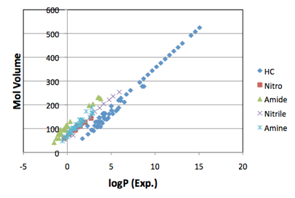
Figure 1‑1 A typical example of linear correlations between MVol and logP. The slopes are the same, with different offsets. The original article at www.pirika.com has many more examples.

Armed with this knowledge it is possible to do a more exact prediction of LogP taking into account the offsets from the different functional groups. This requires the offsets to be additive which, fortunately, they happen to be. With the functional group correction, the correlation between LogP and MVol is very strong:

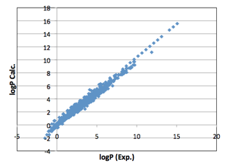
Figure 1‑2 The full correlation of 5,320 experimental LogP values against MVol with functional group correction using the Y-MB functional groups.

Within the typical range of 0-5, the predictions span a range of +/- 1 LogP unit. Given the inevitable uncertainties in the experimental values this is an impressive fit.

 

Azeotropes and Vapour pressures

If a mixture of two solvents were “ideal” then the partial vapour pressures above the mixture would simply depend on the saturated vapour pressure and mole fraction of each solvent.

But we know that in most cases the presence of one solvent tends to make the other solvent “uncomfortable” creating a higher-than-expected vapour pressure. The difference between ideal and real is the Activity Coefficient. So to know everything about the partial vapour pressures of a mixture, the activity coefficients have to be known.

No perfect way has been found to predict activity coefficients, γ. Simple theory suggests that they can be calculated directly from HSP using the formula

Equ. 1‑1 ln(γ)= ln(φ₁/x₁) + 1 - φ₁/x₁ + χ₁₂* φ₂²

where φ₁ and x₁ are the volume fraction and molar fraction of solute 1, φ₂ is the volume fraction of solvent 2 and the parameter, χ₁₂ is given by:

Equ. 1‑2 χ₁₂ = MVol /RT * ((δD₂-δD₂)² +0.25* (δP₂-δP₁)² +0.25*(δH₂-δH₁)²)

In the absence of any better formula, this is a good-enough approximation, but checking against a large dataset of activity coefficients shows that it needs considerable improvement.

At the heart of the problem is that fact that the basic formula does not account for positive interactions between solvents that create activity coefficients less than 1. And a detailed analysis of the failures from predictions of the simple formula show that the biggest deviations typically come about amongst solvents with large δP and δH parameters.

One way to fix this problem is shown by MOSCED – Modified Separation of Cohesive Energy Density. This splits δH into donor/acceptor terms. This seems a good idea. Unfortunately, MOSCED has not become a generally acceptable methodology and some of the more recent fittings of the complex parameters mean that the sum of the cohesive energy terms are often very different from the cohesive energy – in other words, MOSCED has become more of a fitted parameter technique than one rooted in thermodynamics.

In the absence of any breakthrough theory we’ve done a NN fit to a large database of Margules parameters. We have found that the Margules formulation of activity coefficients is more useful than relying on “infinite dilution activity coefficients”, especially as we are often interesting in large mole fraction solubilities.

For Solute 1 in Solvent 2, the activity coefficient γ₁ for mole fraction x₁ (and therefore x₂=1-x₁)is given by:

Equ. 1‑3 Ln γ₁=x₂²(Marg₁₂+x₁(Marg₂₁-Marg₁₂))

 And of course it’s the other way round for Solute 2 in Solvent 1:

Equ. 1‑4 Ln γ₂=x₁²(Marg₂₁+x₂(Marg₁₂-Marg₂₁))

Armed with better predictions across the whole mole fraction range it then becomes simple to calculate the isothermal vapour pressure curves and only slightly more complex to calculate the vapour pressures at the (variable) boiling point of the mixtures from which it is possible to identify important azeotropes.

Solubility

It seems odd to say that you cannot directly predict solubility from HSP! But HSP have always been about relative solubility and have never attempted to issue exact solubility predictions.

However, with some simple equations and some good estimations of key properties, it is possible to predict solubilities directly.

The equation is simple:

Equ. 1‑5 ln(Solubility)= -C + E –A - H

C is the “Crystalline” term, sometimes (confusingly) called the Ideal Solubility. It is the Van ‘t Hoff (or Prausnitz) formula that depends on the difference between the current temperature, T, and the melting point T_m, the Gas Constant R and also on the Enthalpy of Fusion Δ_F.

Equ. 1‑6 C = Δ_F/R*(1/T_m – 1/T)

In other words, the higher the melting point and the higher the enthalpy of fusion, the more difficult it is to transform the solid into the dissolved (liquid) state.

This formula is a simplification which follows convention and ignores some other terms like heat capacities. An even simpler formula, from Yalkowsky, uses just the melting point:

Equ. 1‑7 C = -0.023*(T_m –T)

Recently, Yalkowsky has reviewed the various options for calculating this term, S.H. Yalkowsky, Estimation of the Ideal Solubility (Crystal-Liquid Fugacity Ratio) of Organic Compounds, J. Pharm. Sci, 2010, 99, 1100-1106 and confirms that -0.023*(T_m-T) is good enough. The paper uses Log₁₀ so the printed coefficient is -0.01.

For calculations where T_m≤T, C is zero.

The E term is (combinatorial) Entropy. This is calculated from volume fractions (Phi) and molar volumes.

Equ. 1‑8 E = 0.5*Phi_Solvent*(V_Solute/V_Solvent-1) + 0.5*ln(Phi_Solute + Phi_Solvent*V_Solute/V_Solvent)

It’s worth making an important reminder that molar volumes for solids are not based on their molecular weight and solid density. In the words of Ruelle: “(For a solid) the molar volume to consider is not that of the pure crystalline substance but the volume of the substance in its hypothetical subcooled liquid state.”

A comes from the activity coefficient. The larger the activity coefficient, the more negative A becomes. As discussed above, a simple version of A can be calculated directly from HSP, but the more sophisticated Margules formulation gives better predictions.

H is a Hydrophobic Effect term that is very important for solubilities in water, and somewhat important for solubilities in low alcohols. The calculation follows the method of Ruelle (see, for example, Paul Ruelle, Ulrich W. Kesselring, The Hydrophobic Effect. 2. Relative Importance of the Hydrophobic Effect on the Solubility of Hydrophobes and Pharmaceuticals in H-Bonded Solvents, Journal of Pharmaceutical Sciences, 87, 1998, 998-1014) and depends on r_s*Phi_Solvent*V_Solute/V_Solvent with extra terms depending on how many hydrogen-bond donors (alcohols, phenols, amines, amides, thiols) are on the solute and whether the solvent is water, a mono-alcohol or a poly-ol. The value r_s is 1 for monoalcohols and 2 for water and, for example, ethylene glycol. It is 0 for all other solvents. If the solvent is water and the solute contains alcohol groups, there are special parameters depending on whether the alcohols are primary, secondary or tertiary. There is a further refinement (not included in this version) which discounts some of the solute’s hydrogen bond donors if they are likely to be internally bonded. The important thing about the Ruelle formula is that solubility in water depends almost entirely on the size of the solute – bigger molecules are simply less soluble than smaller ones. Their explanation is more sophisticated than the simple idea that bigger molecules disrupt more hydrogen bonds, but the simple intuition isn’t a bad approximation. They show that for “simple” molecules (one’s without too many –OH groups) spanning a huge range of solubilities, a first principles formula based on MVol, with no fitting parameters, does an excellent job at prediction.

The complication is that the E, A and H terms all depend on the volume or molar fraction which is precisely what you are trying to calculate, so there is an iterative process involved until the equation balances.

Although the output of most interest is the real solubility, it is very instructive to see the effect of the different terms, so the HSPiP modeller shows the C, E, A and H terms. For all solvents that aren’t water or alcohols H is zero. For water the H term, not surprisingly, can be very large. But because of water’s small molar volume, the E term can also be large. Because the A term can also be large, water solubility is hard to judge a priori because it can involve the (partial) cancellation of large numbers.

A very helpful way to think through solubility issues has been provided P. Bennema, J. van Eupen, B.M.A. van der Wolf, J.H. Los, H. Meekes, Solubility of molecular crystals: Polymorphism in the light of solubility theory, International Journal of Pharmaceutics 351 (2008) 74–91. The equations below can be switched on and off in the Crystalline Solubility Theory modeller and plots can be chosen as x v T (so both are in “normal” units) or as ln(x) v 1/T which is the van’t Hoff plot which gives a straight line (added as a reference to the plot) for ideal solubility, making it easier to see the effects of switching on and off the different parameters. The Yalkowsky approximation is included for reference.

For the ideal solubility case the mole fraction solubility x is given by the equation we have used earlier:

Equ. 1‑9 Ln(x) = Δ_F/R*(1/T_m – 1/T)

However, this assumes that the heat capacity Cp of the virtual liquid at temperature T is the same as that of the solid. In general the heat capacity is higher so ΔCp is positive. This happens to increase the solubility, sometimes to a surprisingly large extent via:

Equ. 1‑10 Ln(x) = Δ_F/R*(1/T_m – 1/T) + ΔCp/R [T_m/T – ln(T_m/T)-1]

If regular solution theory is used then there is an additional term that depends on ΔH_mix, the enthalpy of mixing and ΔSmix, the enthalpy of mixing. If this is positive (i.e. the solute and solvent do not like to be together) then the solubility is reduced, if it is higher (there is some positive interaction between them such as donor/acceptor) then the solubility is increased. The formula including all three terms is then:

Equ. 1‑11 Ln(x) = Δ_F/R*(1/T_m – 1/T) + ΔCp/R [T_m/T – ln(T_m/T)-1] – (ΔH_mix -TΔS_mix)/R [(1-x)²/T]

HSPiP allows you to play with these terms. Clearly the dominant effect is still the melting point – the higher it is (and the higher the enthalpy of fusion) the lower the solubility, but the surprisingly large Cp effect and some assistance from a negative heat of mixing can at least fight against the low solubility that a high MPt generally brings.

The fact that x is on both sides of the equation for heat of mixing effects leads to some strange plots for high values of  ΔH_mix. The strange plots are not realistic because they happen to represent violations of Gibbs phase rule. Whether they represent “oiling out” effects is a matter that can be followed up by those who read the paper referred to above.

 

E-Book contents | HSP User's Forum