Chapter 35, A Short History of the Hansen Solubility Parameters

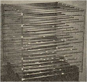
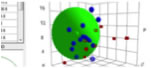
Figure 1‑1 Where it all began: the initial HSP values for the 88 solvents were determined the hard way on this equipment in Hansen’s lab. δD is in the direction of the rods which had rings at regular intervals.  δD = 14.9 and δP= δH=0 is at the lower foremost corner where there is a white label for n-hexane [14.9, 0, 0]. Magnets with wires glued to them were used to plot data for the provisional values for the three parameters using colored beads.

 

The Main Track

I was born in Louisville, Kentucky. I graduated from the University of Louisville, Speed Scientific School with a B.Ch.E in 1961. Wanting to continue for a doctorate, I was in the process of working for a Ph.D. at the University of Wisconsin, Madison, having gotten a Masters degree, but wanting to take a year in Denmark before having to “settle down” with the advanced degree. My father came from Denmark, arriving in the US in 1929, and my mother’s family came to the US in the late 1800’s. Not really knowing what had been done to accommodate a useful study, I arrived in Denmark to find that I was able to stay not one year, but two years, provided I wrote a thesis to obtain a degree then called “teknisk licentiat”. I accepted and delivered the thesis in exactly 24 months as planned. I knew from earlier correspondence that I could either work on an automatic process control project or on a question in the coatings industry related to why solvent is retained in polymer films for years. I chose the latter.

When I was finishing the work for the technical licentiate degree in 1964 [1] there were a couple of Master’s candidates working as a team on the use of solubility parameters in the coatings industry at the Central Research Laboratory of the Danish Paint and Varnish Industry. I advised them occasionally and this lead indirectly to the development of what are now called Hansen solubility parameters. I was formally associated with the Technical University of Denmark (at that time called Den polytekniske Læreanstalt) where Prof. Anders Björkman arranged for my stay. The actual work was done at the above laboratory led by Mr. Hans Kristian Raaschou Nielsen, in a rather small room with a slanting ceiling on the uppermost floor at Odensegade 14, Copenhagen Ø.

As stated above, my licentiate thesis was to explain how solvent could be retained in coatings for many years. It was thought that this was caused by hydrogen bonding. I showed solvent was retained because of very low diffusion coefficients. It is especially difficult to get through the surface of a coating where there is essentially no solvent and diffusion coefficients are very low. The diffusion controlled phase followed a phase where most of the solvent initially present freely evaporated. In the meantime it was necessary to account for the hydrogen bonding capability of the test solvents, because of what was believed at the time. The work of Harry Burrell [2] provided the basis for selecting test solvents. He qualitatively ranked a number of solvents according to weak, moderate, or strong hydrogen bonding. The licentiate thesis did not treat solubility parameters as such, dealing only with diffusion and film drying, since it was not hydrogen bonding or the solubility parameter that had anything to do with the problem, other than allowing solution in the first place. There was, however, established a battery of solvents and knowledge about solubility parameters at the laboratory, and the Master’s candidates were to further the development of this area.

An article by Blanks and Prausnitz appeared [3] and I advised the students to make use of the new method of dividing the Hildebrand parameter into two parts, one for dispersion interactions and one for what was called “polar” interactions. They did not do so, having already gotten into their study and they needed to finish as planned, being short on time. After I turned in my licentiate thesis for evaluation, I looked at their experimental data using two dimensional plots of the dispersion parameter versus the new “polar parameter” as described by Blanks and Prausnitz. I could see there were well-defined regions of solubility on the plots. For some polymers there were bad solvents within the good region of the 2D plots. For other polymers these were the good solvents. The other ones had now become bad. The one group was largely alcohols, glycols, and ether alcohols, with the other being ketones, acetates, etc. It seemed logical to use a third dimension, pushing the bad solvents into another dimension, and this was the basis for the original terminology “The Three Dimensional Solubility Parameter” that was used in the original publications in 1967 [4-7]. I followed the rule that the sum of energies in the (now) three partial parameters had to equal the total reflected by the Hildebrand parameter, recognizing that Blanks and Prausnitz were correct as far as they had gone. No one up to that point had recognized that the hydrogen bonding effects were included along with the polar and dispersion effects within the Hildebrand parameter itself. The Hildebrand parameter is based solely on the total cohesive energy (density) as measured quantitatively by the latent heat of vaporization (minus RT). Hydrogen bonding was considered too special to allow such a simple approach as the HSP division of the total cohesion energy into dispersion, polar, and hydrogen bonding contributions. Efforts prior to Blanks and Prausnitz had used the Hildebrand parameter together with some more or less empirical hydrogen bonding parameter, for example, in efforts to make useful solubility plots. Barton’s handbooks review these earlier attempts in an exemplary manner, and as usual I refer to his handbooks for these developments rather than repeating their content [8,9].

Prior to the public defense of the licentiate thesis, I visited the US, returning to Denmark for the big day. While in the US I visited the Univ. of Wisconsin to try to establish a continuation of the earlier studies based on the promising work on solubility parameters that had become obvious to me, at least. Professors Ferry (of WLF equation fame), DiBenedetto, and Crosby, all would accept me, but only working on projects for which they already had funding. After return to Denmark for the public defense, Prof. Björkman urged me to stay on to complete a Danish dr. techn. (similar to D.Sc.). I accepted, and found a room with a relative, rather than in the student dormitory where I also got indoctrinated into the student life of the time in Denmark. 1967 was a big year. My father had to come to Denmark twice, once for a wedding and once for the public defense of the dr. techn. thesis, an event he could not quite believe would happen. He himself was a chemical engineering graduate from the same school, and knew that not that many got so far. It is my belief that because of the privileges provided by Prof. Björkman (just do it at your own speed), that I am the youngest (29) to ever have been awarded this degree. The requirements of the technical doctorate are that one presents and defends his or her own ideas in a written publication. This must then be defended in a very formal (coat and tails) public event with official opponents that must not last longer than 6 hours. There was newspaper coverage with an audience of 125, filling every seat in the auditorium. My official opponents were Prof. Anders Björkman (polymers), Prof. Bengt Rånby (polymers), and Prof. Jørgen Koefoed (physical chemistry). The event lasted about 4 hours. As an indication of the iconoclastic nature of this thesis, Prof. Koefoed challenged in advance that I could not assign the three parameters to formamide, and that the mixture of equal molar amounts of chloroform and acetone must give deviations. I then proceeded to assign the three parameters to formamide by calculation and experiment, and tried to experimentally test all of my test solutes in the acetone/chloroform mixture. There were no errors in the predictions. The thesis was accepted.

I initially had a three dimensional model as shown in the opening figure made with metal rods at equal spacing supported by clear poly(methyl methacrylate) sides. There were rings on the rods at uniform intervals. The D parameter was in the direction of the rods, varying from 7 to 10 in the old units (cal/cc)^½. Each of what ultimately became about 90 solvents was represented by a given magnet to which a wire was glued so that given points in the space could be labeled. A small green bead was place on the tip of the wire for a good solvent and a small red one was used for a bad solvent. One could thus make a 3D solubility plot for each of the 33 solutes. These were mainly polymers chosen to potentially have such widely different solubility properties as possible. If a given solvent seemed to be giving consistent errors, its P and H parameters were adjusted, keeping the D parameter constant, and the magnet with wire tip was moved. This trial and error procedure clearly showed the value of the three dimensional methodology. Tests were made with mixtures of non-solvents. If such a mixture dissolved a given solute, the solvents had to be on opposite sides of the region of solubility. It they did not they were on the same side. This method was used to confirm the parameters for as many of the solvents as was reasonable. I then took a solvent and willfully placed it on the wrong side of the system and started all over. It became obvious that the system was inverting, so it was concluded that these numbers were reasonably good, but would probably need revision at some time. Publications were prepared.

The first revision came rather quickly in 1967 from the insight of a colleague at the Danish laboratory, Klemen Skaarup. He found the Böttcher equation for the polar parameter, did a lot of calculations, and plotting, and the initial values were revised accordingly. The changes involved in these revisions were not that great as can be seen from the earlier publications. Mr. Skaarup was also responsible for the first use of the “4” in the key equation of the methodology, finding this would give spheres rather than spheroids for the solubility regions. The “4” was generally considered as empirical for many years thereafter.

These “three dimensional” concepts were reported in three articles in the Journal of Paint Technology and in the dr. techn. thesis, which also included an expanded section on diffusion in polymers and film formation, in 1967 [4-7]. I have reviewed the dr. techn. thesis many times, and have found nothing wrong with it yet. It can be found as a PDF file on my website www.hansen-solubility.com.  

Just prior to the public defense of the dr. techn. thesis I corresponded with Prof. Prausnitz to see whether the studies could be continued with him. The response was that there was no funding.  I then took a job at the PPG Industries Research and Development Center in the Pittsburgh area. These eight years were very rewarding with a remarkably inspiring leadership “Making Science Useful” (Dr. Howard Gerhard and Dr. Marco Wismer). There were many confirmations that the methodology could be used to great advantage in practical situations. I was popular in the purchasing department during the solvent crisis (oil crisis) where one had to buy whatever was available on the spot. I could immediately on the phone confirm whether or not a given solvent could be used and the usual testing was not done. Shiploads of solvent were bought on this basis only.

Dr. Alan Beerbower at Esso (now Exxon) was just waiting for me, as he said it himself, and took up the developments in the 1967 publications in many areas as can be seen in our article in the Encyclopedia of Chemical Technology [10] and in his many publications on a variety of topics, often related to surfaces, lubrication, and surfactant behavior, for example in [11,12]. He developed group contributions, adding to what was known at that time (citing Fedors), that I used and reported in the handbooks [13,14]. It was Dr. Beerbower who first used the term Hansen plot as far as I know. Dr. Beerbower authored a brochure for Esso that appeared in 1970 entitled “Parameters of Solubility”. Here is the cover of that handbook and inside, Beerbower’s reference to the Hansen principle:

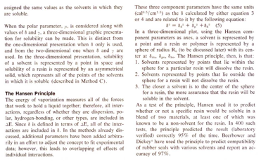
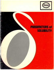
Figure 1‑2 Perhaps the first reference to Hansen (component) parameters in the literature from Beerbower’s 1970 handbook and a gratifying confirmation of 97% accuracy for prediction of solubility.

 

 I have put one of his figures in the Handbooks [13,14]. In the Second Edition this is on page 338. This figure also appeared in Beerbower’s publications but I got it only as a personal communication. Sometime after the appearance of the article in the Encyclopedia of Chemical Technology [10] in 1971, where the terminology was not changed, probably because I did not use it, Hansen (solubility/cohesion) parameters replaced the “three dimensional” terminology on a more general basis. Van Krevelen did not like three dimensional systems, but did the group contributions for the “solubility parameters” anyway in his “Properties of Polymers” from 1975, so the change in terminology was not complete at this point in time.  Barton’ handbook in 1983 used the Hansen parameter terminology as cited below. I have never had contact with Van Krevelen. A US Coast Guard project in 1988-9 studying chemical protective clothing brought me back on track in terms of adding a significant number of solvents to the database. I was to find solvents for testing that could permeate a PTFE body suit after having established a correlation for those solvents that had been tested. As it turned out there were indeed quite a few solvents that permeated the PTFE suit  that were characterized by molar volumes less than about 60 cc/mole and monomers with terminal double bonds that could be somewhat larger [13,14] (see the figure on page 247 of the second edition of the handbook). I actually initially had a technician looking at the published Van Krevelen group contribution approach early in this project, before realizing that I had to do it myself with the Beerbower group contributions that I had gotten as a private communication. The Van Krevelen and Hoy approaches are now outdated, being surpassed by the work of Stefanis and Panayiotou (See for example Chapter 3 in the Second edition of the handbook or their other publications. HSP estimates by the S-P statistical thermodynamics methodology are also included in HSPiP). Even this has been outdated very recently by the work of Dr. Hiroshi Yamamoto in the HSPiP where it is called the Y-MB method for Yamamoto Molecular Breaking. Both Hiroshi and I independently found that one did much better when using larger “groups” for the still larger molecules, even to the extent of directly using the existing HSP of multifunctional molecules as a whole as a single group.

The superiority of modern computers that are capable of working with huge databases to generate correlations with rapidity and flexibility stands in contrast to what was done earlier. The first calculations for dividing the latent heats into partial solubility parameters were done using a slide rule. Indeed there were computers that could have helped with this at the time, but this cost money, and the data were very scattered in the literature. The first computer program to calculate the HSP spheres from experimental data was probably that at PPG Industries around 1968. My lab there was set up to routinely determine the experimental data that helped to optimize solvents and to predict compatibility. Safety and the environment were emphasized. A similar program was available at the single, central computer of the Scandinavian Paint and Printing Ink Research Institute, and later on my son, Kristian, wrote the same type of program for use at our home on a Commodore 64. This typically took about 20-30 minutes to calculate the HSP sphere from data on approximately 40 solvents. Much of the data in the handbooks was done on this computer.

I left PPG in 1976 to become director of the Scandinavian Paint and Printing Ink Research Institute, being invited to do so largely at the suggestion of the Swedish participants (Prof. Bengt Rånby, Prof. Sven Brohult). This was a Danish-Swedish organization at the time, but when I left 10 years later, Finland and Norway were also part of the Nordic cooperation. These 10 years also led to further progress and development of knowledge in the area, mostly in the further characterization of materials and from applications in industry. Research as such was not permitted at my final place of employment, FORCE Technology, so the developments were not as extensive as what might have been expected. I did manage to write the first edition of the handbook (at home) [13], and to search for and find what I believe to be theoretical justification for the “4” in the key HSP equation. The Prigogine corresponding states theory of polymer solutions has the “4” in the first term of the free energy equation, but only when the geometric mean is used to predict interactions between unlike molecules. Other averages give quite different results.  The HSP approach also uses the corresponding states approach wisely chosen by Blanks and Prausnitz, comparing data for a given solvent with corresponding states data for its look-alike hydrocarbon solvent (homomorph). Blanks and Prausnitz inherently also assumed the geometric mean for the molecular dipole-dipole interactions. To this day there are those who protest inclusion of the hydrogen bonding as is done in the Hansen methodology. These interactions are considered non-symmetrical with only symmetrical interactions being describable by the solubility parameter theory. It seems that if dipolar molecular interactions and the orientation involved are included, there should be no objection to include the hydrogen bonding molecular orientation. The fact that the dispersion, dipolar, and hydrogen bonding energies sum to the total cohesion energy for thousands of chemicals is difficult to dispute as well.    

One might wonder when usage of the HSP concept first took off. I cannot answer this with any certainty. I have concentrated on my direct responsibilities in industrial environments, trying to follow the relevant literature as well as possible. I sense that industrial use has been extensive even very shortly after the 1967 work appeared. These uses are rarely published. I was shown the number of citations of my publications as a function of year, and it was clear that something happened around 2000, after the first edition of the handbook appeared. The academics, who must certainly give the majority of reference citations, first really took interest the past 10 years or so. The key persons involved in the development and spreading of the concept almost all had direct or close industrial ties including myself, Beerbower, Hoy, Van Krevelen, Abbott, and Yamamoto. The academics would necessarily include Patterson and Delmas (who showed negative heats of mixing were found as expected from solubility parameter theory) and Panayiotou and coworkers who put the hydrogen bonding cohesion energy into a statistical thermodynamics context with success. The following is a typical academic reaction from the late 1960’s  to my early work. This is taken from a series of lecture notes/thesis from Denmark. I prefer not to name the author here. Quote: The “theory” is applied to a very complicated systems, such as solutions of macromolecules in polar and hydrogen-bonded solvents and solvent-mixtures. Even though the method seems to have some technical value, the theoretical basis is extremely weak. It is only to hope that serious work with the solubility parameter theory is never judged with such empirical methods in mind”. End of Quote. This sums up the majority of the academics early views on “the three dimensional solubility parameter”, and there are presumably still many who hold this view or something similar to it judging from the lack of knowledge in the area that I find during my journal review activity. To my knowledge, with only a few notable exceptions, there has been only very limited entry into classrooms at universities, although there have been many Ph.D. thesis that have made use of the concept. The full social and economic potential of this methodology will not be realized until universities include this in introductory courses. After all, the concept is very simple and very useful.

The Side Track

For those who want to know a little more of what went on behind the scenes here are some more personal and informal comments made in response to questions from Prof. Abbott.

The Hoy solubility parameters just sort of appeared some time after I was at PPG. One had to write to Union Carbide to get a booklet with the tables. The tables were arranged according to alphabetical order, evaporation rate, total solubility parameter, polar solubility parameter, hydrogen bonding solubility parameter, and boiling point. The first booklet appeared in 1969.  These values were also later revised for some solvents. Quoting from a letter dated May 23, 1988, from Union Carbide accompanying a booklet dated 1985 - “Enclosed is a recent copy of the “Hoy Tables of Solubility Parameters” you requested. It is basically the same as the 1975 edition, but some updating of the data was done in 1981. Ken sends his greetings to you and looks forward to seeing you in Athens. Signed R.L. Bradshaw.” The Hoy parameters appeared in Barton’s handbook from 1983 [8]. They apparently gained wide usage in the USA because there were data for many solvents not in my published work and perhaps also because of the major influence and support of Union Carbide. Once established in a given location, there has been a tendency for interest in them to continue. I have never fully understood how these were calculated. The Hoy dispersion parameter was consistently lower than that found from the corresponding states approach, and the expansion factor alpha appeared in both the polar and hydrogen bonding terms, so I felt they were not independent. The dispersion parameter was found by subtracting the polar and hydrogen bonding contributions from the total. I have always warned not to mix the Hoy parameters with the original HSP. The Hoy parameters appeared as well in the first edition of Barton’s handbook (1983) with the title “Hildebrand and Hansen Parameters for Liquids at 25°C, Determined by Hoy as Described in Sections 5.9 and 7.1”. The Hansen parameter terminology was therefore fully introduced at this time. I met Ken Hoy on many occasions and fully respected his work, also in other areas. I have used the Hoy total parameter on many occasions, and religiously went through the table in the Barton handbook from 1983 using the Hoy data for Hildebrand parameters and molar volumes/density for many solvents in a transfer to my own HSP. Only a few solvents (larger hydrocarbons) were not included in my list.

I gave 5 presentations at Gordon Research Conferences starting in 1967 at the Coatings conference. Here I met Harry Burrell who gave a talk on hiding without pigment (using light scattering from microvoids), but he had dropped further solubility parameter work by that time. There was also a talk by Crowley, Teague, and Lowe from Tennessee Eastman describing their three dimensional approach to polymer solubility which had appeared the year before. They used the Hildebrand parameter, the dipole moment, and an experimental (empirical) hydrogen bonding parameter that I think was found from mixing solvents to precipitate polymers, much like Kauri Gum is precipitated from n-butanol solution to find the KB values. These were not generally used and are hardly mentioned in the Barton handbooks, but the thinking was in the right direction. I was admittedly a little disturbed as to where they had gotten their idea, having sent a manuscript to the Journal of Paint Technology earlier, presumably early in 1966. I withdrew the manuscript for some reason, perhaps for reasons of knowledge gained in the meantime. I had a feeling the Eastman people had gotten access to this report, but was assured by Crowley that they had not been aware of it.  It was at this Gordon Conference that PPG became aware of my work, thus leading to employment.

At an Adhesion Gordon Conference I was confronted in the discussion after the presentation by a comment from Fred Fowkes, an outstanding surface chemist. He said that I must have invoked Phlogistine theory (everything is made from earth, fire, water, and air) to assign a hydrogen bonding parameter to toluene. I did not know what this was at the time (A Google search on the word just confirmed the spelling and meaning), but I responded that the experimental data clearly indicated that even toluene had some hydrogen bonding character, although I could not precisely evaluate it. I could see it was less than 2, but greater than 0, so I took 1, not being too far off in any event. The units here are (cal/cc)^½. At a Polymers conference my talk led to a subsequent discussion lasting about 1½ hours. The group was split between the academics, who thought it to be bunk, and the industrialists, who loved it. I got the traditional Amy Lifshitz award for promoting discussion, which meant I had to drink a glass of a clear yellow liquid at the Thursday night meeting, having earlier described the attributes of the most common form of saturated urea/water as used through history for various purposes as a solvent and swelling agent. An academic exception was Prof. Tobolski who came to me the next day with support, relating his own problems with the existing Establishment (Flory in particular, who delayed publication of a paper to get his own in first). As an aside, I might mention that I have been told that there were three different schools who did not think well of each other at all. There was one school in favor of Hildebrand (Univ. of California), one school in favor of Prigogine (Univ. of Florida), and one school in favor of Flory (Stanford). My own personal response to this is that I have never knowledgably had problems with any of them. What they all lacked was quantification of the hydrogen bonding effects. Another academic, Prof. Donald Patterson, whom I met on several occasions, was also very supportive and explained things along the way at key points in time to help me along. A paper with his wife (Delmas) showing negative heats of mixing were not only found, but they were found as predicted by solubility parameter theory, was a  true milestone. This work was very timely and decisive in changing many minds away from “empirical” to at least “semi-empirical”. A major objection I often met was how can both negative and positive heats of mixing be accounted for by solubility parameters? The Pattersons cleared this up as mentioned above. Another major question, also discussed briefly above, was that Hildebrand assumed the geometric mean rule for calculating the interchange energy between two different kinds of molecules, and that another rule was probably valid for hydrogen bonding. My answer to this has been that polar interactions were accepted as following the geometric mean rule. Since these are molecular and involve molecular orientation, I could not see why the molecular hydrogen bonding interactions should be any different in this respect. In addition all of the many success stories using HSP, where the geometric mean had been assumed following Hildebrand, have convinced me that this is the correct way to do it..

My last experience with Gordon Conferences was also something special. Percy Pierce, my very close colleague at PPG, had invited me from Denmark around 1980, and I was on after the lobster dinner on Thursday evening. This particularly bad timing did not help, because I showed pictures of brain scans. The Danish doctors, whom I believed, (but am no longer completely sure of what side effects there may have been in their patients), claimed to have found and shown brain shrinkage because of solvent exposure. I found out later that this caused (very) great concern in the coatings industry, but no one could talk about it because of the rules of the Gordon conferences. Anyway, I have never been to a Gordon Conference since. One might question why?

I have not attended international conferences outside of the Nordic countries since about 1986. The lack of salesmanship of this kind probably delayed the acceptance in the academic community. This would have been done on vacation and at my own expense and just seemed out of the question under the circumstances. The Danish Establishment has not been particularly supportive in the past few decades. The major grants are controlled by academics for the sole use of academics. I have only been significantly employed in industrial environments. There have been some government incentives for cooperation between industry and academia in an effort to force the cooperation between the more academic endeavors and industry. As an example I will cite the 5 year grant for cooperation between my employer (FORCE Technology), the Risø National Laboratory (now a part of the Technical University), and 9 Danish companies. (This was popularly called MONEPOL in the Danish acronym) The consortium worked on Polymer Degradation. This resulted in about 25 publications including two Ph.D. theses. The first year was led by my immediate supervisor, who then decided he could not manage it. I was cautiously asked whether I would take over and did so with great pleasure for the next 3½ years. I could not finish the last half-year, having unwillingly left my job, because of not accepting a forced reduction in working days.

There have been many papers on solubility parameters, cohesive energy density, cohesive parameters, interaction parameters, and the like, and Barton did a great service in his thorough collection and reviews of these. The last Barton handbook appeared in 1991. I have never had the resources and/or time to do this sort of thing, but there are many significant reports that have appeared in the interim, the results of which should be collected. I did manage a handbook that appeared in 1999, but time requirements restricted it mainly to what I had been doing. When I discovered the “4” in the Prigogine theory in 1998, I decided immediately that this had to be published. At the same time I had written so many journal articles, that I reasoned all I had to do was the equivalent of writing a few more journal articles and put it into a book. Fortunately CRC thought this was a good idea as well. Donald Patterson was very helpful at this time, as acknowledged in the handbook.

Having written the handbooks [13,14] has made me more cautious about handbooks. There was indeed no review, and I could write whatever I wanted to. In the second edition of my Handbook I helped the others who contributed where I could, but my own writings appeared without review, if that term is used appropriately. Rest assured that I still stand by what was written.

It is sometimes asked why approaches such as UNIFAC and HSP have never been coordinated. I can only say that my own attempts to initiate discussions to this end have never been reciprocated. My own ability to influence matters was usually restricted by the fact that I worked in industry. My attempts to remain in or re-enter academia and therefore have the time and resources to work on such issues were not well-received. All I can say is that I have done the best I can with the resources available to me.

One small example of this is that a grant to me at the Technical University of Denmark was stopped after 10 months instead of the 2 years I was told would be the case (writing a book on diffusion). This ultimately led to employment at FORCE Technology. The main import of my concepts on diffusion in polymers was thusly delayed for over 20 years. A recent article in the European Polymer Journal (Hansen, C. M., "The significance of the surface condition in solutions to the diffusion equation: explaining ‘anomalous’ sigmoidal, Case II, and Super Case II absorption behavior", European Polymer Journal, Vol. 46, 651-662 (2010) summed up what I would have written in the late 1980’s. Some few additional but significant pieces of information have appeared in the interim, but the main message is the same (the surface condition must be considered to understand the so-called anomalies).

Finale

In more recent times the second edition of the handbook was written in semi-retirement [14]. It was recognized again that many others had now done significant work, both academic and industrial, and several of these contributed to this edition of the handbook in their own areas of expertise (John Durkee, Georgios Kontogeorgis, Costas Panayiotou, Tim Poulsen, Hanno Priebe, Per Redelius, and Laurie Williams). I was grateful for these contributions, without which the second edition would not have appeared. Their work advanced acceptance of the HSP methodology.

I met Prof. Abbott through a Danish company called CPS (Chemical Products and Services). CPS grew based on the production of more environmentally acceptable cleaners already in the late 1980’s,  primarily for the serigraphic printing industry. I had gotten a special government grant for the fledgling company for the development of the first series of these cleaners. There were patents with examples based on HSP. This company was bought by Autotype in England, who were later bought by MacDermid in the USA. Prof. Abbott led the technical activities at Autotype, and naturally appeared as a member of the board of CPS. On one occasion I rapidly solved a problem using HSP where Prof. Abbott was having some difficulty. He had not been looking in the third dimension (the D parameter). This then led to his development of suitable software and ultimately to where we are with HSPiP in, as I write this, December, 2010.

The most recent and extensive contributions to the HSP theory and its practical applications appear in the HSPiP (Hansen Solubility Parameters in Practice) eBook and software. This was started at the suggestion of Prof. Steven Abbott, with Dr. Hiroshi Yamamoto soon joining in. These two have an unbelievable work ethic. The volume and quality of what has appeared recently, and is still appearing on a regular basis, is amazing. All of the significant methods for estimating HSP are included for those who may wish to continue their use. The Stefanis-Panayiotou (S-P) method based on a statistical thermodynamic treatment as described in the second edition of the Handbook, has already been more or less surpassed in volume and accuracy by the Hiroshi Yamamoto’s molecular breaking method (Y-MB), supported by the extensive data, numerous comparative correlations, and simple software application (just enter SMILES or MolFiles). I am very thankful that what was started in the years 1964-1967 will survive and be used for a great many purposes for the benefit of society and the environment.

References

1)    Hansen, C.M., The Free Volume Interpretation of the Drying of Lacquer Films, Institute for the Chemical Industry, The Technical University of Denmark, Copenhagen, 1964,

2)     Burrell, H., A solvent formulating chart, Off. Dig. Fed. Soc. Paint Technol, 29(394), 1159-1173, 1957. Burrell, H., The use of the solubility parameter concept in the United States, VI Federation d’Associations de Techniciens des Industries des Peintures, Vernis, Emaux et Encres d’Imprimerie de l’Europe Continentale, Congress Book, (The FATIPEC Congress book), 21-30, 1962.

3)    Blanks, R.F. and Prausnitz, J.M., Thermodynamics of polymer solubility in polar and nonpolar systems, Ind. Eng. Chem. Fundam., 3(1), 1-8, 1964.

4)    Hansen, C.M., The three dimensional solubility parameter – key to paint component affinities I. – Solvents, plasticizers, polymers and resins, J. Paint Technol., 39(505), 104-117, 1967.

5)    Hansen, C.M., The three dimensional solubility parameter – key to paint component affinities II. Dyes, emulsifiers, mutual solubility and compatibility, and pigments. J. Paint Technol., 39(511), 505-510, 1967.

6)    Hansen, C.M., The three dimensional solubility parameter – key to paint component affinities III. Independent calculation of the parameter components. J. Paint Technol., 39(511), 511-514, 1967.

7)    Hansen, C.M., The Three Dimensional Solubility Parameter and Solvent Diffusion Coefficient, Doctoral Dissertation, The Technical University of Denmark, Danish Technical Press, Copenhagen, 1967. PDF file can be found on www.hansen-solubility.com.

8)    Barton, A.F.M., Handbook of Solubility Parameters and Other Cohesion Parameters, CRC Press, Boca Raton FL, 1983.

9)    Barton, A.F.M., Handbook of Solubility Parameters and Other Cohesion Parameters, 2^nd ed., CRC Press, Boca Raton FL, 1991.

10) Hansen, C.M. and Beerbower, A., Solubility Parameters, in Kirk-Othmer Encyclopedia of Chemical Technology, Suppl. Vol., 2^nd ed., Standen, A., Ed., Interscience, New York, 1971, pp 889-910.

11)  Beerbower, A., Boundary Lubrication – Scientific and Technical Applications Forecast, AD747336, Office of the Chief of Research and Development, Department of the Army, Washington, D.C., 1972.

12) Beerbower, A., Surface free energy: a new relationship to bulk energies, J. Colloid Interface Sci., 35, 126-132, 1971.

13) Hansen, C.M. Hansen Solubility Parameters: A User’s Handbook, CRC Press, Boca Raton FL, 1999.

14) Hansen, C.M., Hansen Solubility Parameters: A User’s Handbook, 2^nd ed., CRC Press, Boca Raton FL, 2007.

 

E-Book contents | HSP User's Forum