In earlier editions, this was a short chapter. It was about adhesion and its main aim was to counter naive ideas that adhesion was “all about surface energy”. The chapter has now expanded to bring in some serious polymer physics of adhesion and has been extended to include polymer solution viscosity and a return to basic polymer solubility. The logic of combining them in one chapter will hopefully become clear.

On first reading you may well want to abandon this chapter once the polymer physics starts to get difficult. But if you come back to the chapter from time to time you’ll find that the concepts in the later sections really throw a lot of light onto many of the issues you face when using polymers and solvents. As is so common in science, insights from the discussion of one problem (e.g. polymer adhesion) can be helpful in an apparently unrelated area (e.g. the disturbing ability of polymer solutions to become very viscous with small changes in conditions).

First let’s turn to the adhesion between two polymer formulations. Whether you are interested in classical polymer-to-polymer adhesion or getting an ink to stick to a polymer surface, the considerations are the same.

Sticking together

It turns out that HSP can provide insights that help us distinguish between three types of adhesion. The first type of adhesion, based on surface energy, is insignificant. The second, delightfully named “nail adhesion” is quite common and (as those who prefer to screw things together already know) quite unreliable. The third is the real adhesion for those situations where things must stay stuck together – the wing on your aeroplane or the legs on your chair.

Real adhesion is not based on surface energies

There is a common misconception that adhesion is all about surface energies. It is well known that a polymer of low surface energy such as polyethylene has low adhesion, but once corona treated has (a) a high surface energy which allows an applied coating to flow out rather than bead up, and (b) good adhesion. From these facts the conclusion is that the increased adhesion to the polyethylene is due to the high surface energy.

There is a very simple disproof of this view of adhesion. The surface energies of PVC film and PET film are identical. Yet it is very easy to get printing inks to stick to PVC and very hard to get them to stick to PET.

There is another common half-truth about adhesion. It is well-known that roughened surfaces tend to have stronger adhesion than smooth surfaces. The common explanation for this is that there is more surface area for adhesion on the roughened surface. This is true, but the effect is small. A typical “rough” surface like this probably has only 10% extra surface area:

Figure 0‑1 A normal rough surface has a small increase in surface area

To double the surface area you need a surface of a dramatic roughness (a high 1:1 aspect ratio):

Figure 0‑2 It takes extreme roughness like this to double the surface area and double the adhesion due to surface energy

The main reason why roughened surfaces increase adhesion has to do with crack propagation. If there is a smooth interface and a crack appears, all its energy can be transmitted straight along the interface and the crack moves along swiftly, destroying adhesion. If there is a rough interface, much of the crack energy is sent into directions away from the crack so the crack does not propagate.

The myth of surface energy being important for adhesion comes from some good, simple science. The work of adhesion Wa of two surfaces can be simply calculated:

Equ. 0‑1 Wa= γ * (1 + Cosq)

Where γ is the surface energy and q is the contact angle of the second material with the first. If the surface goes from wetting (q = 0º) to non-wetting (q = 90º) the work of adhesion changes only by a factor of 2. This is a small effect when we’re talking about real-world adhesion where differences are factors of 100’s.

The real explanation for the dramatic increase of adhesion to polyethylene after corona treatment is the fact that the polyethylene crystals are broken up at the surface and an open polymer surface is available to interact with whatever you are trying to stick to the surface. The meaning of “interact” is explained below. The functionalisation of the surface by the treatment is a surprisingly small effect – often only 1 in 100 surface carbon atoms has been oxidised. This is enough to allow good wetting of an applied coating (an important effect) but largely insignificant in providing real adhesion

Before we come on to the key science of real adhesion, it’s worth mentioning the Gecko effect. There have been many bad explanations of how a gecko can climb up a smooth surface. It turns out to be very simple. Van der Waals forces of two surfaces in intimate contact are more than strong enough to support the weight of a gecko. So all the gecko needs to do is make sure there is plenty of surface contact. The feet are designed with multiple levels of compliance, ensuring that there is every chance for bits of the feet to be in contact with as much of the surface as possible. In simulations, it hardly makes much difference if the feet are high or low surface energy. Going back to the issue of crack propagation and surface roughness, it’s clear that cracks fail to propagate along the many interruptions in the surface contact of the gecko.

But the key thing about gecko adhesion is that it is perfectly useless for “real” adhesion. The gecko can lose adhesion with a mere flick of its foot. And of course this is vital because the gecko has to be able to walk. If adhesion were too good it would be stuck forever. So gecko adhesion is closer to “scientific adhesion”. It’s elegant, functional, explainable with simple surface physics, but ultimately useless for most areas of adhesion that are of practical interest to humans. It’s common, for example, to have layers of ink with good “gecko-like” adhesion but which peel off all too easily when put under real-world test conditions.

We shall soon put some numbers to all this which will show that surface-energy adhesions of  ~0.1J/m² are a factor of 100-1000 too small to explain real adhesion.

In what follows we largely ignore adhesion of polymers to non-polymers such as metals. However, a later discussion about chemical bonding between surfaces (of particular relevance to metal/polymer bonding) shows that entanglement issues play an important and little-known role.

HSP to the rescue

When dealing with polymers, real-world adhesion comes mostly from intermingling of polymer chains. The more the chains are intermingled, the harder it is to pull them apart when stress is applied at real-world speeds. It’s like untangling a ball of string. If you pull the string very slowly and carefully it’s possible for it to slide out from the tangles. But if you pull it quickly the tangles tighten upon themselves making it impossible to move. In scientific terms if the polymers are above a “critical entanglement limit” then adhesion is strong.

To get polymer chains to entangle (and stay entangled – i.e. we’re ignoring temporary tricks such as solvents compatibilizers) they have to be thermodynamically more stable when extended as opposed to closed in upon themselves. If you try to mix two polymers with very similar HSP (think of the extreme case where the HSP are identical because the polymers are identical) then they will entangle readily (provided there is some kinetic boost such as heat or solvent). Two dissimilar polymers will simply not mix.

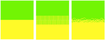
Figure 0‑3 No intermingling (surface energy only, poor adhesion ~0.1J/m²), straight intermingling (“nail” adhesion ~1J/m²) contrasted with entanglement (real adhesion 100-1000J/m²)

It’s obvious from the picture that the polymer system on the left will have poor adhesion. The one in the middle has good interpenetration of the polymers so you might think that the adhesion will be OK – but it won’t be much good. We’ll see that it takes the situation on the right with strong entanglement before decent adhesion is obtained.

The measure of HSP similarity between two polymers is the HSP distance between them (taking into account their respective radii). A short HSP distance is a strong indicator of the potential quality of adhesion, providing they have a kinetic chance to mix via solvent or thermal treatment. The effect of chain length is more difficult to predict. Short chains will not have strong entanglement, but they are easy to intermingle. Long chains will have very strong entanglement, provided they’ve had sufficient exposure to solvent or heat. Similarly, linear chains are easier to entangle but easier to disentangle than branched chains. And in a complex polymer, it may happen that the average HSP is not suitable for compatibility but certain segments (side-chains, blocks) are more compatible, provided they are given the chance to come to the surface. Sometimes it requires a compatible solvent to get the correct segments to flip to the surface in order to bond with the other surface. But even though there are many subtleties, the HSP distance is a crucial component of adhesive thinking.

(We note in passing that these entanglement issues are highly relevant to Environmental Stress Cracking, where higher molecular weight variants/mixes of a polymer are often more resistant to ESC).

The HSP radii of the two polymers encapsulate one other element of the problem. Polymers with small HSP radii are, for various reasons such as high molecular weight or high crystallinity, harder to access, so require a closer HSP match.

The polyethylene example now makes more sense. Wetting and film retention alone does not assure acceptable adhesion, but by breaking up the crystal structure through the corona treatment, interaction with whatever you are trying to stick becomes possible. By adding some modest (oxygenated) functionality, the HSP compatibility with many adherents is increased. There’s a final sting in the tail about corona treatment for increasing adhesion. The destruction of the surface which is a desirable feature can be taken too far. You then have polymer rubble on the surface. Adhesion of your ink to this rubble might be quite good. But it is building a house on sand. It’s well-known, for example, that PET corona treatment can create rubble and considerably reduce adhesion in many systems, making it a difficult judgement call if you find that for your system the adhesion is enhanced (once more, by breaking up the crystalline domain of bi-axially oriented PET). How can you tell if that enhancement is permanent or something that’s going to fail because the pile of rubble falls apart?

The polymer physics of adhesion

The description above is OK as far as it goes, but it’s a bit on the vague side. Let’s get deeper into the polymer physics. For those who want a masterful modern summary of the physics, try the review by Richard P.Wool, Adhesion at polymer–polymer interfaces: a rigidity percolation approach, Comptes Rendus Chimie 9 (2006) 25–44.

A useful starting point suggested by Professor Wool is “nails” adhesion. His paper is a classic and well worth reading: Richard P. Wool, David M. Bailey, Anthony D. Friend, The nail solution: adhesion at interfaces,  J. Adhesion Sci. Technol., 10, 1996, 305-325. Take two blocks of wood and nail them together. The more nails N you have, the longer, L, they are and the higher the friction µ between the nail and the wood, the greater the adhesion. In fact the Fracture Energy =0.5µNL². If you do the calculation for typical short polymer chains across an adhesive bond (as shown in the middle image of the diagram above), the fracture energy turns out to be something like 1J/m². This is higher than any reasonable surface energy bonding energy of ~0.1J/m². But “real” adhesion is in the 100’s to 1000’s of J/m², so “nails” adhesion is rather close to useless. If you want two blocks of wood to really stay together you use screws instead of nails. For polymers you can’t have screws, but you can have entanglement.

There’s a precise description of “entanglement” and it is therefore possible to calculate some “critical entanglement parameters”.

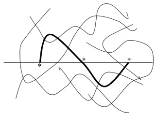
Figure 0‑4 The classic “Wool” diagram (with permission) showing the three crossings necessary for entanglement.

A polymer chain can be said to be entangled across an interface if it crosses it three times. One or two crossings are equivalent to one or two nails, only three (or more) crossings ensure entanglement.

It turns out there is a critical length required for a polymer chain to be able to wander back and forth that many times. This can be expressed as a critical molecular weight M_c or a critical length L_c or critical “radius of gyration”  R_gc (they are, of course, inter-related). The formula for M_c and L_c are:

Equ. 0‑2 M_c=31(bz/C)²jM₀C_∞

Equ. 0‑3 L_c=b_s(M_c/6M₀)^½

Unfortunately you need to know quite a lot about your polymer before you can do the calculation. b is the average bond length, b_s (often confusingly shown as b) is the statistical or “Kuhn” length, z is the number of monomers per unit cell of size C, j is the number of bonds along a monomer (e.g. 2 for PS, PMMA, PE… and 12 for PC), M₀ is the monomer molecular weight. C_∞ is the “characteristic ratio” for your polymer, a number that encapsulates the stiffness of the chain and which varies between about 2-18.

A useful collection of these parameters can be found in L. J. Fetters, D. J. Lohsey and R. H. Colby, Chain Dimensions and Entanglement Spacings, Physical Properties of Polymers Handbook 2^nd Edition, Chap. 25, 445-452, 2006.

Here are some typical values deduced from that and other references:

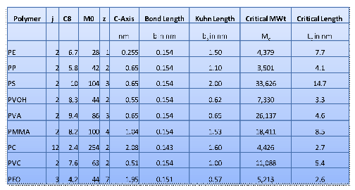
Figure 0‑5 Typical examples of the key parameters for entanglement calculations.

When it comes to adhesion across a polymer boundary these critical values are important. The two polymers form an interlayer width, d. If d<L_c, the critical length, then you only have nails adhesion. So the question arises, what is the typical value of d?

There is a well-known formula for this:

Equ. 0‑4 d=2b/(6χ)^½

where b is the statistical bond length and χ is the interaction parameter. It’s interesting to note that χ is sometimes assumed to be a specific Flory-Huggins term, but in fact Hildebrand derived it from pure solubility parameter considerations and it was later shown (especially by Patterson) that (a) the Hildebrand and the Flory-Huggins χ’s are essentially the same and (b) they both contain approximations that happily tend to cancel out and give good results. Hansen took the Hildebrand definition and put it into its now-familiar form:

Equ. 0‑5 χ=MVol/RT*((δD₁-δD₂)² + 0.25*(δP₁-δP₂)² + 0.25*(δH₁-δH₂)²)

Now we have our χ it seems as though we can easily predict adhesion from our HSP! Unfortunately it’s not that simple. There is significant disagreement in the literature about the use of χ in these calculations, not least because a standard way of measuring χ using Small Angle Neutron Scattering (SANS) is itself open to much dispute.

Note that the MVol in the formula is the molar volume of the polymer (not of the monomer unit). If you quadruple the molecular weight then the MVol is quadrupled and the interlayer width is halved (a 1/MVol^½ relationship). This means that the laws of physics are against you. As you increase the molecular weight to approach or exceed L_c, the interlayer width decreases making it harder for d>L_c. That’s one of the reasons it’s so hard to get really good adhesion between polymers.

Getting d≫Lc is important and the Number of Entanglements, N_e=d/L_c is a very significant number. There are good experimental data showing that bond strength is small when N_e<1 (i.e. below the critical entanglement limit) and then has a linear dependence on N_e>1. So if d=2L_c the bond strength is double that of d=L_c.

The Adhesion calculator in HSPiP can only be seen as indicative. The  χ  calculation itself is uncertain, and you have to enter estimates for many parameters to calculate d. Furthermore you are calculating the interface for two polymers with only one b_s and MVol. And you are likely to be dealing with polymers of broad molecular weight distributions rather than the idealised single molecular weight implicit in the theory and used in the experiments that have proven the theory. But as a guide to the sorts of issue you face when designing an adhesive interface it seems to be much better than having no tool at all. What is certain is that a smaller HSP distance will give better adhesion if the following three conditions are met:

·      The molecular weights of both polymers exceed Mc for critical entanglement

·      The calculated d>Lc

·      There has been sufficient bonding time and mobility for the entanglement to take place

The last factor is the great unknown. If you are melt-bonding two polymers then the time for them to diffuse to distance d depends on t^¾ MWt^-7/2. The problem is that it’s relatively easy for the polymers to diffuse by “Rouseian” dynamics but these, by definition, do not involve entanglement, they just give you nail adhesion. As you become entangled you are in the domain of Reptation dynamics (“a snake sliding down a tube”) which are slower with a large dependence on MWt. The “obvious” way to increase entanglement is to lower the viscosity via a good solvent. Unfortunately, the more solvent that’s present, the further apart the polymer chains are so the less likely they are to entangle. This is not to say that solvent-based entanglement is bad, it’s simply to point out that polymer physics are against you if you’re not careful.

A logical way to attain a good interface between two polymers is found frequently in the world of real adhesives. A di-block co-polymer made from the two polymers will obviously be compatible on each side of the interface. The trick is to make sure that each block is long enough to be firmly entangled within its own polymer, otherwise you have di-block nail adhesion which is not as effective. The classic study on this (Creton et al, Macromolecules, 25, 3075, 1992), using PS-PVP di-blocks showed a fracture energy of ~5J/m² when the PS was above its entanglement length and the PVP was below it, with all the fracture failure on the PVP side. Once the PVP exceeded its entanglement length the fracture energy rose to ~100J/m².

Polymer physics gets you again

In a paper Polymer-Solid Interface Connectivity and Adhesion: Design of a Bio-based Pressure Sensitive Adhesive, most conveniently found online at http://www.che.udel.edu/pdf/WoolPaper.pdf Wool and Bunker provide a startling demonstration of the importance of entanglement. Suppose you have a surface (e.g. a metal) with functional groups –Y and you want to bond a polymer with functional group –X which forms a strong –X-Y- bond.

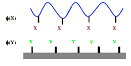
Figure 0‑6 What are the optimum φ(X), φ(Y) for good adhesion? Less than you would think!

It seems obvious that the stronger the bond and the larger the fraction of –X and –Y bonds (φ(X), φ(Y)), the stronger the bond will be. “More” is obviously “better”. Yet Wool (and others) have shown that a φ(X)>~1% leads to a rapid decrease in bond strength. How can this be?

The key to this puzzle is the mode of failure. Below this critical φ(X) the failure mode, not surprisingly, is adhesive: the polymer pulls away from the surface. Above the critical value the failure mode is cohesive: a thin layer of polymer remains on the surface. The reason for this is entanglement, or, rather, loss of it. As you get more and stronger –X-Y- links, the more the surface layer of polymer gets flattened onto the surface and therefore the less it can entangle with the rest of the polymer partly because of reduced mobility and partly because the chains do not extend far enough into the bulk in order to entangle. This is not a small effect. For their particular adhesive the bond strength goes from 250 J/m² at 1% to 50J/m² at 1.2%, a catastrophic reduction in practical adhesion for just a small increase in φ(X).

There is no HSP message in this small section – we simply find this to be a fascinating bit of science which is surprisingly little-known.

A quick way to test for contamination

All the adhesion science is worth nothing if your surfaces are contaminated. So a quick way of testing for contamination can be very handy. Although this chapter stresses that the common myth about surface energy being important for adhesion is out by a factor of >1000, surface energy tests can be an excellent way to identify contaminants. Although one can use surface-energy pens (“Dynes pens”) there is an even easier way. It was developed by the same Hansen who developed HSP and is an official Nordtest Poly 176: (www.nordicinnovation.net/nordtestfiler/poly176.pdf ). A set of vials contain ethanol/water mixes varying from pure ethanol (surface tension=22 dynes/cm) up to pure water (72 dynes/cm). Starting from the ethanol end of the range, drops from each are placed on the test surface till one is found that does not spread. That, then, is a guide to the surface energy of that surface. This is not a way to measure the surface energy, it is simply a guide. The point is that if you know that you get a good bond with a surface that spreads drops up to 46 dynes/cm (10.9:89.1 ethanol:water) and your test piece spreads only up to 36 dynes/cm (23.4:76.6) then there’s something wrong with your surface.

Hansen has used the technique to identify contaminants on many items including wind-turbine blades and the cement lining of a major tunnel. In both cases, just a few drops of ethanol/water were sufficient to identify problems that could have had major long-term consequences. Ethanol/water is not an aggressive solvent mix for most surfaces so the results are seldom confused by surface damage from the solvent.

The test isn’t perfect. If your 46 dynes/cm is covered by a 46 dynes/cm contaminant then you’ll never know. But very often the contaminant will be some sort of lower surface energy oil and the test will reliably detect it.

Polymer viscosity

This section doesn’t have much to do with adhesion. But because so many of the considerations are similar, and because the calculations in the software are on the same modeller, we’ve included this summary here. You may find the following a little frustrating. There seem to be so many parameters and assumptions to hold on to and there seem to be many uncertainties in the estimates. That seems to be the nature of this literature. It is very difficult to find papers that pin down all the key variables in one go and then link them to experimental values. We’ve done our best. As ever, if the HSPiP community can provide better ways of doing this, we’ll be happy to update this text and the program.

First we need to define R_g, the Radius of Gyration of the polymer. It is given by a formula that is similar to the Mc calculation above. The C_∞, j and M₀ values are given for a range of polymers in the software and b can be assumed to be 0.15nm if you don’t have a better value to hand.

Equ. 0‑6 R_g0=b [C_∞Mj/(6M₀)]^½

Unfortunately, R_g depends on how “happy” the polymer is within the solvent. This formula gives the R_g for a polymer in a neutral solvent – i.e. one with neither positive nor negative polymer/solvent interactions. Such a solvent is termed a theta solvent and so we call this value R_g0.  As the solvent gets better, the polymer tends to expand so R_g is larger. The traditional way is to say that R_g=Rg₀ α² where α is an expansion factor. Unfortunately there is little agreement on how to know α. In HSP terms, polymer “happiness” is defined by the RED number. When RED=1 the polymer is on the border between happy and unhappy – i.e. at or near the theta point and the R_go from the above formula is used. As the RED reduces, the R_g increases (the polymer likes to be in the solvent). Note that RED is in solubility parameter units. Chi and the interaction coefficient are in energy units. A RED of 0.9 converts to a chi effect of 0.81 by the squaring process. In other words the reduction in RED is more important than a linear reduction. We’ve chosen a simple estimate of this effect that works adequately with data from the classic known polymers. It’s saying that for a good solvent, R_g goes as Mw^1.6, for a theta solvent it goes as Mw^1.5 – but with a higher constant of proportionality. Mw is the weight averaged molecular weight. For these sorts of calculations, Mn, the number averaged molecular weight is not so useful.

Equ. 0‑7 R_gRED=R_g Mw^{(1.6 - 0.1 * RED)} / Mw^1.5  (1 + 1.5 * RED) / 2.5)

Because the viscosity effects are highly dependent on Rg, we decided to let you decide which value to input. So we output Rg₀ and R_gRED to give you an indication of likely R_g values; you then use your scientific judgement in providing an input value.

An alternative way to estimate R_g0 is to use handbook tables of R_g0/Mw^½. We’ve provided a selection of these values in the program. Obviously you need to multiply them by Mw^½ to get the R_g0 which you can then compare to the value calculated in the program.

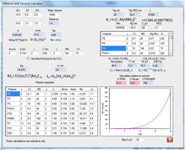
Figure 0‑7 The complexities of polymer adhesion and viscosity made as simple as we possibly can

We must at this point take a side-track into the connection between the definition of a theta solvent and RED number. At first we hit an intellectual problem. A theta solvent corresponds to a RED=1 (Chi=0.5) where, by definition, we have no solubility. Yet polymer physicists happily make solution measurements in theta solvents so there has to be some solubility. The fix for this problem arises because the definition of a theta solvent applies to a polymer of infinite molecular weight. As the molecular weight gets smaller the polymer starts to have some solubility. In other words, RED=1 for an infinite polymer means RED<1 for a finite polymer. The theory of all this is discussed in the next section, but in short, a RED of 0.9 for a polymer of MVol=10,000 in a solvent of MVol=100 corresponds to a theta solvent. For a polymer of 100,000 the RED is 0.97. Given the many assumptions behind these corrections, for the purposes of the viscosity calculations, a RED of 1 is assumed to be equivalent to a theta solvent, with the understanding that the finite polymer is inside the border of the sphere and can therefore be dissolved in sufficient amounts to make theta-solvent measurements. Errors in other estimates far exceed the errors in this RED=1 approximation.

The viscosity of a dilute polymer solution (we will define “dilute” in a moment) depends on the intrinsic viscosity [η]₀ and the concentration. At very dilute solutions the specific viscosity is given by  [η]₀C (Zimm), where specific viscosity is (η_p- η_s)/ η_s and C is the concentration (in the software C is in g/l). In other words, the specific viscosity is the viscosity of the solution containing the polymer η_p corrected for the viscosity of the solvent η_s. By extrapolating specific viscosity to zero concentration you obtain [η]_0. We can calculate [η]₀ in units of l/g via:

Equ. 0‑8 [η]₀=5 AvR_g³/Mw

An alternative way to estimate [η]₀ is to use handbook tables of K₀ where [η]₀ =K₀Mw^½, where the “0” indicates that these are values for a theta solvent. Handbooks may also provide K and a values for calculating [η] in good solvents where [η] = KMw^a and a is higher than the 0.5 for theta solvents (typically 0.6-0.7). It’s impractical to include these in HSPiP so use the given K₀ values to cross-check (multiplying by Mw^½)  the intrinsic viscosity calculation using the R_g for a theta solvent, then change to a good solvent and assume that the enhanced R_g translates to a correctly enhanced [η].

Polymer chains start to interact even in dilute solutions. Because of this the general “dilute solution” formula for the traditional way of reporting polymer viscosities, η_p/ η_s is given by the following formula.  For simplicity the ratio η_p/ η_s will be called η in the following;

Equ. 0‑9 η_dilute=1+[η]C+0.4([η]C)²

Above a certain critical concentration, C^*, the solution ceases to be “dilute” and Rousean dynamics take over and the (hypothetical) Rousean viscosity is given by:

Equ. 0‑10 η_Rouse= ([η]C)^1.3

C^* is the point at which the polymer “blobs” start bumping into each other. It is calculated as

Equ. 0‑11 C^*=Mw/(AvR_g³)

Where Av is Avogadro’s number (6.022E23).

The Rousean domain doesn’t last long. As the concentration increases, the polymers start to get entangled and viscosity starts to rise dramatically. This critical concentration depends on Ne (the number of monomer units in a critical entanglement molecular weight M_e). Ne= M_e/M₀, where M_e is 1/3 the M_c we’ve calculated above. So:

Equ. 0‑12 N_e=(M_c/3)/M₀

Knowing N_e we can then calculate the critical entanglement concentration, C_e. We called the Rousean domain hypothetical because the entanglement effects start to kick in fairly quickly (at C>0.5C_e) and it seems hard to spot true Rousean viscosity because at 0.5C_e you can be close to the dilute limit.

Equ. 0‑13 C_e=N_e^(3v-1)/(6.6/C^*)

The 3v-1 term would be a simple 0.5 in a theta solvent where the polymer/solvent interactions are neutral. But as you go into good solvents it gets easier to entangle. For classic polymers in good solvents, the exponent term, v ~0.585, making 3v-1=0.755, a big increase on 0.5. As a practical heuristic we’ve proposed the following for v:

Equ. 0‑14 v=0.585-(0.085*RED)

With all these equations we can now predict viscosity over the entire range of polymer concentrations. If you play with the Viscosity modeller you will find that small changes in v or in Rg can make large changes to the calculated viscosity. This makes it very hard to be sure that you’ve got good predictions. You will also notice that the three graphs plotted (dilute, Rousean, entangled) don’t overlap. This is because no entirely self-consistent description of all three domains seems to exist and in any case the Rousean curve is hypothetical. The point of the graph is to show the general form of typical polymer viscosity behaviour.

If you find this disconcerting, the reality of polymer solutions is that relatively small changes (molecular weight and/or its distribution, concentration, temperature, solvent blend) can produce relatively large changes in viscosity, so the errors apparent in the lack of overlaps are likely to be smaller than the effects arising from, say, molecular weight distribution.

If you start going to high RED numbers (>1) and large concentrations you will find that the calculations become decidedly odd. But remember, at RED>1 you cannot get high concentrations, so the calculations are irrelevant!

There’s one more key fact. The viscosity we’ve calculated after all this hard work is only the zero-shear viscosity. Predicting the non-Newtonian changes in viscosity at higher shear is, perhaps, a challenge for future editions of HSPiP.

But the point of this section is not to provide a 100% reliable viscosity predictor (as far as we know such a thing doesn’t exist). Instead we’re giving you a modeller where you can see the general effects of molecular weight, solvent compatibility (RED number), concentration etc. and therefore better understand what’s going on in your own system. If you are already an expert in the field, then this section won’t be necessary. If you are not an expert then hopefully the calculations and graphs will provide you with some insights that will help you better understand the literature of polymer viscosity and apply it to your own polymer/solvent system.

Because we’ve taken a giant side-track into polymer physics, we might as well finish off with some thermodynamics that tidy up some loose ends in the explanation of the polymer sphere radius.

Really understanding polymer solubility

In the “minimum theory” chapter we described how solubility was about thermodynamics. But we didn’t give a thermodynamic formula for this. It’s now time that we did. We use the convention that “1” refers to the solvent and “2” the polymer and we use V₁ and V₂ for the molar volumes and ϕ₁ and ϕ₂ for the volume fractions. It’s more normal in thermodynamics to use mole fractions, but because of the huge disparity in molar volumes, the numbers don’t look very helpful. Because of this disparity the “x factor” is introduced. This is simply x= V₂/V₁.

So now we can introduce the formula for the partial Gibbs free energy of  the solvent on dissolving a polymer:

Equ. 0‑15 ΔḠ ₁=RT [ln(ϕ₁) + ϕ₂(1-1/x) + Distance² ϕ₂² V₁/(4RT)]

The first two terms are the entropy of mixing, the third term is the enthalpy of mixing. The factor of 4 is there because of the factor of 4 in the (δD  term of the) HSP Distance calculation. The combination of the first two terms is usually called the Flory-Huggins entropy.

Because negative free energies are good for solubility, it’s important to note that the 2^nd and 3^rd terms are both positive. So solution is only possible because of the ln(ϕ₁) term. As you dissolve more polymer (ϕ₂ increasing), ϕ₁ decreases so ln(ϕ₁) gets more negative – the classic entropic driving force. But of course the ϕ₂ term gets ever larger, fighting against solution. Only if x≤1 does the ϕ₂ term cease to be a problem. But x is always large so the 1-1/x term is always >0. For an infinite molecular weight polymer, 1/x=0 so the ϕ₂ effect is maximum. As the polymer gets smaller the ϕ₂ effect reduces (though not by a lot) and the chance of being soluble increases. Non-intuitively, a larger solvent means a reduced ϕ₂ effect, so in this respect small solvents are bad.

The Distance² factor in the third term reminds us that the smaller the HSP distance, the higher the chance of dissolving. The sphere radius then comes from when the Distance is large enough for the 3^rd term to produce a positive ΔḠ. As we will shortly see, this distance is between 7 and 8, which is what is found experimentally for a large number of polymers. The reasons for variations around this number will shortly emerge. And because the 3^rd term also includes V₁, we will soon see that small solvents are nearly always a good thing, as intuition and practical experience shows. In other words, the 3^rd term solvent size effect (small is good) usually outweighs the ϕ₂ effect (small is bad).

It’s not obvious how all these terms work out in practice. So we’ve made a Polymer Solution Theory modeller that lets you input the key properties: V₁, V₂ and Distance. The ΔḠ is then plotted over a ϕ₂ range of 0-0.3. The scale for ΔḠ is deliberately made small so that the details can be seen around the important 0 line. In particular, the classic case of a 10,000:100 polymer:solvent gives an inflexion point at a critical value which translates to a Chi value of 0.605. For an infinite polymer, this point of inflexion moves to 0.5, which is why a Chi of 0.5 is seen as the definition of borderline solubility (theta solvent). Because of the relationship between Chi and Distance for an infinite polymer a Distance of 7.05 provides the boundary of solubility. This can be calculated from first principles, but you can show this for yourself using the modeller.

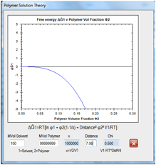
Figure 0‑8 For an “infinite” MVol polymer the thermodynamics of solubility go critical at Chi=0.5 or a Distance of 7.06.

 

For the 10,000 polymer (as shown in the figure below) it’s a distance of 7.77. The ratio 7.06/7.77 ~ 0.9, which is why we stated above that a RED of 0.9 suffices for a real polymer compared to an infinite polymer.

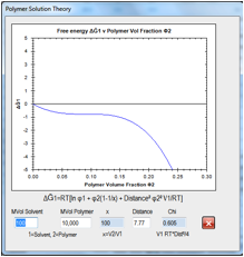
Figure 0‑9 For a 10,000 MVol polymer in a 100 MVol solvent, the thermodynamics of solubility go critical at Chi=0.605 or a Distance of 7.77. That’s why we often say that a typical polymer HSP radius is 7-8.

Remember, this is all theory based on many assumptions. It is well-known, for example, that the Flory-Huggins entropy is not a perfect approximation. Real solvents and polymers can’t be calculated with this precision and some spheres have a radius of 10 and some of 5.

Let’s first see why we might have a small radius. There’s an important term missing from the ΔḠ equation. If the polymer is crystalline then (thermodynamically speaking) before it can dissolve it first has to melt. This “crystalline” energy (sometimes confusingly called “ideal solubility”) is discussed in the Predictions chapter but the formula is simple:

Equ. 0‑16 C = Δ_F/R*(1/T_m – 1/T)

where Δ_F is the enthalpy of fusion and T_m is the melting point. For normal crystalline solids these terms are readily known. For polymers things are seldom so crystal clear. We are therefore making no attempt to predict it. However, what is obvious is that the larger the value of C the smaller the Distance needed to ensure solubility. That is why highly crystalline polymers have such small radii. Polyethylene is a classic example. Its HSP mean that finding a compatible solvent is not at all hard. But solution experiments using polyethylene normally take place at ≫100ºC so that the (1/T_m – 1/T) term becomes small enough to allow the solvent to dissolve the polymer. The reason that you find solvents such as Decalin being used for polyethylene is not because they have special solubility parameters, but because they have a high enough boiling point to be able to do experiments at 130ºC.

Rather satisfyingly we can come back to the corona treatment of polyethylene. The disruption to the crystallinity at the surface means that the C term becomes small so that ordinary solvents at low temperature have a chance of interacting strongly with the top few nm of the polymer film, provided their Distance from (perhaps slightly functionalised) polyethylene is not too large.

One possible reason for a large radius comes from the following inverted reasoning.

Backward thinking

It’s obvious that if the polymer isn’t soluble in the solvent then the solvent isn’t soluble in the polymer. This “obvious” fact is completely wrong. The “x-factor” above explains why. If the 1 and 2 of solvent and polymer are swapped then the thermodynamics stay the same but the important ϕ₂ (1-1/x) term is transformed. For a 10,000 polymer and the same solvent, x is now 0.01 so the ϕ₂ term is multiplied by 1-100 which is decidedly negative, so this term strongly aids solution.

In other words, even though the polymer may be hardly soluble in the solvent, the solvent may be highly soluble in the polymer. This very important point is often missed.

For example, it illuminates the discussions on diffusion into polymers. Even though the polymer may never dissolve in the solvent, there is still a chance that the solvent will dissolve in the surface of the polymer, starting the diffusion process. The HSP distance is still very important – the smaller the distance the larger the amount of solvent that will dissolve in the polymer – even though classic HSP solution experiments might show that the polymer is effectively insoluble in the solvent. You can (as discussed in later chapters) determine HSP via diffusion/permeation experiments. Solvents that are no good for dissolving the polymer can still permeate reasonably, so the sphere based on these experiments can be large.

This effect also explains why the HSP spheres of solvent swelling experiments can be larger than spheres of true polymer solution.

This doesn’t mean that the diffusion/permeation or swelling spheres are “wrong”. You as the scientist choose your definition of the sphere according to your purpose. If you are interested in polymer diffusion/permeation or polymer swelling then such a large sphere is correct. You only go scientifically wrong if you try to use the numbers from one domain (swelling) in another (polymer dissolving in the solvent).

This backward thinking isn’t just for polymers. A classic example is that the solubility of water in hydrocarbons is hardly affected by the MVol of the hydrocarbons.  Yet the solubility of hydrocarbons in water is highly MVol dependent. The best way to understand this is via the classic solubility equation. At first there seems some confusion as the Distance term now contains V₂, the solute, whereas in the polymer case it was V₁. The reason is that in the polymer case we were calculating the partial Gibbs free energy of solution, with the focus on V₁. In the classic solubility case we are calculating the activity of the solute, so the focus is on V₂.

Equ. 0‑17 ln(a₂)=ln(mf₂) + Distance² ϕ₁² V₂/(4RT)]

Here we have the activity of solute 2 in solvent 1. We use mf₂ for mole fraction rather than the conventional “x” to avoid confusion with the use of x above.

When we are trying to dissolve water in hydrocarbons, V₂ is that of the water and because Distance² doesn’t vary all that much between hydrocarbons, solubility does not change much.

When we try to dissolve hydrocarbons in water, V₂ is that of the hydrocarbons and the activity increases (solubility decreases) as they get larger.

Finally, although in the case of water dissolving in hydrocarbons MVol makes little difference, we need to return to the general rule that smaller solvents are better for polymers.

This can easily be checked from the Polymer Solubility Theory modeller. Just change MVol Solvent from 100 to 90 (whilst keeping the HSP Distance the same) and a situation of critical solubility becomes one of good solubility:

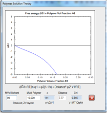
Figure 0‑10 For the same HSP Distance, if the solvent MVol decreases, the free energy curve ceases to be critical and the polymer is likely to dissolve.

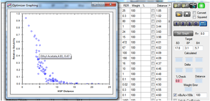
The Solvent Optimizer contains a simplified version of the solubility/distance equation. If you enter the Radius of your polymer, the “Relative Solubility” is calculated as exp(-Distance² V₂/Rterm) where we’ve assumed a constant ϕ₁² and use an “Rterm” which is proportional to the chosen Radius (and contains the RT term). A larger Radius means a smaller negative exponential and therefore a larger Relative Solubility. With the mouse you can read off the various solvent values from the graph.

Summary

Congratulations if you’ve reached this far. Our view of this chapter is that it poses three further challenges.

1. The “easy” challenge lies in understanding the formulae and getting used to playing with the modellers in order to work out what’s going on. We’ve peppered the modellers with the formulae so that when you get a surprise (as we often do) you can work out why changing parameter A affects parameter B which in turn affects the output C in a way you didn’t expect.

2. The “hard” challenge is to find ways to map the theory into one’s scientific and technical work. Even though the theory is complex enough, it still contains lots of simplifying assumptions and, as we admit, only gives “indicative” numbers. Yet we’ve found in our own real-world work that the modellers and the ideas behind them have proved crucial in disentangling (pun intended) complex issues. They are particularly good in providing a common numerical language that a cross-functional team with varying expertise in physics, chemistry and analytical science can use to build a fuller picture of what’s going on in their system.

3. The final challenge is for ourselves, with the help of the HSP community, to build further on these foundations and increase the range and depth of the predictive power derived from the theory.

 

E-Book contents | HSP User's Forum