DIY
For many of the modellers within HSPiP
properties are calculated automatically by inputting SMILES data.
Many users aren’t too familiar with
SMILES so this form of input might appear useless. But we can say two things.
First, SMILES are far easier than you might think and very quickly you get used
to them. Second, it is usually very easy to find the SMILES for a chemical of
interest to you with a simple web search such as MyChemical Smiles. Wikipedia, for
example, includes SMILES for most of its chemicals. You can also find them in
ChemSpider where you enter the chemical name or the CAS#. Even better for the
long term is to find the molecule using InChIKeys – see the Y-MB section for
more details.
Excellent guides to SMILES can be found
at
http://en.wikipedia.org/wiki/Simplified_molecular_input_line_entry_specification
and
http://www.daylight.com/dayhtml/doc/theory/theory.smiles.html
and you can test out SMILES at
http://www.daylight.com/daycgi/depict
See http://www.pirika.com/NewHP/PirikaE/Smiles.html for a typical example of generating a Smiles in a freeware
molecular drawing package and bringing it into HSPiP.
Simple linear molecules using these rules
are
CCO Ethanol
CC=O Acetaldehyde
C=CC Propene
CC#N Acetonitrile
Branching is shown with brackets, with
the branch being to the atom to the left of the bracket:
CC(C)C(=O)O Isobutyric Acid
Where the first (C) is the side methyl
group and the (=O) is the double-bond oxygen of the carboxylic acid.
Cyclic structures are shown by numbers
that indicate where a ring starts and ends. So
C1CCCCC1 Cyclohexane
has a “1” after the first carbon to say
“the ring starts here” and a “1” on the 6th carbon to say “and this is joined
to the other C1”.
Aromatics can be shown in two ways:
C1=CC=CC=C1 Benzene
or
c1ccccc1 Benzene
n1ccccc1 Pyridine
o1cccc1 Furan
It gets more complex with –NH members of
aromatic systems and an [NH] symbol is used
n1c[nH]cc1 Imidazole
Finally (for this simplified guide),
cis-trans isomers across double bonds are shown as / and \
Cl/C=C/Cl Trans
di-chloroethene
Cl/C=C\Cl Cis
di-chloroethene
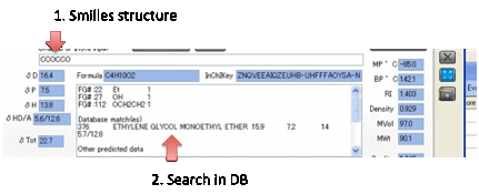
InChI
Because we believe that the relatively
new InChI (International Chemical Identifier) standard for
describing molecules is going to be of great future importance, we output the
“standard” InChI and InChIKey.
These are created with the “No
Stereochemistry” option so they are the simplest possible outputs. Importantly,
if you use the first 14 digits of the InChIKey as the search string on places
such as ChemSpider (probably the best one-stop-shop for information on a
chemical) then you are guaranteed to get the correct matches. InChIKeys are
unique identifiers created from the InChI so unlike CAS# they are directly
traceable to specific molecules and there is only one InChIKey (well, the first
14 digits) to a molecule. The reason we emphasise the first 14 digits is that
they will find all variants of a given molecule, independent of
stereochemistry, isotope substitution etc. Once you start using InChIKeys for
searches you’ll wonder how you ever survived without them.
For a useful quick guide to InChI, visit http://en.wikipedia.org/wiki/International_Chemical_Identifier
If you input an InChI then we output the
Smiles for your reference.
DIY utilities.
There is no one, universal, simple,
accurate way to calculate HSP from the molecular formula. This is frustrating
for all of us who use HSP. Until such a method appears, the only alternative to
measuring them directly yourself is to make do with a range of techniques which
you can mix and match to reach your own best judgement on the HSP values. This
really is a DIY (Do It Yourself) approach to HSP.
However, because of the power of Y-MB we
recommend this as your basic HSP calculator.
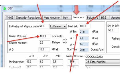
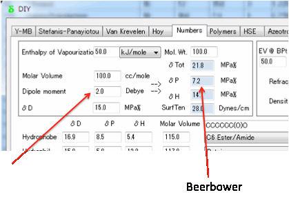
1 Numbers & Surfactants
You need to enter the Enthalpy of
Vaporization (ΔHvap) in
kJ/mol and the Molar Volume in cc/mole. The Cohesive Energy, E is then
calculated as:
E= ΔHvap - RT
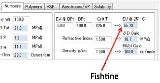
ΔHvap at 25 = ΔHvap at Tb
*[(1-298.15/Tcr)/(1-Tb/Tcr)]0.38
If you don’t know Tcr then a
reasonable guess is Tcr=Tb+225
From these δTot (the sum of the three components,
i.e. Sqrt(δD² + δP² + δH²) can be calculated directly and
accurately.
There are arguments in favour of using
the more complex Böttcher equation (see Equation 10.25 in the second edition of
the Hansen handbook, for example), but as it is unlikely that you will have the
accurate numbers for the dielectric constant, refractive index and dipole
moment required for that equation, the Beerbower equation seems adequate.
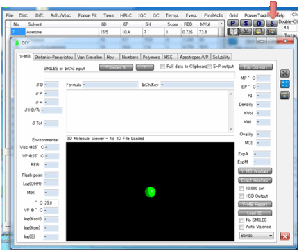
2 Y-MB
Dr Hiroshi Yamamoto is an expert on
fitting large datasets using Neural Network techniques. He has taken the full
HSPiP Solvent Data.hsd set plus thousands of other compounds and provided an
optimal Neural Network and Multiple Regression fit and has then tested it
extensively on a wide variety of compounds – this is made easy because he has
provided the means to go straight from molecular descriptor (Smiles, (standard)
InChI or 3D file such a .mol) to HSP.
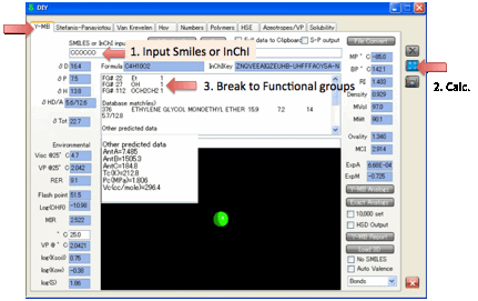
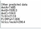
In addition to the HSP δD, δP, δH, δTot (and also a Check δTot which is from the sum of the 3 HSP),
Y-MB gives you molecular weight, molecular formula and estimated RI, MPt and BPt, each calculated via a Neural Network algorithm using
literature data for each of the parameters. Values for Antoine Coefficients and critical
parameters
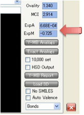
are also estimated for your convenience and added to the output text box. Ovality and MCI (Molecular Connectivity
Index) are added for convenience as they are now used in some of the property
estimation schemes. The MCI, for example, significantly improves estimation of
BPts. Even more parameters are available from the Y-Predict Power Tool.
ExpA and ExpM are important for accurate
calculations of HSP values at temperatures other than 25ºC because the HSP values
depend in a complex way on the change of density caused by thermal expansion.
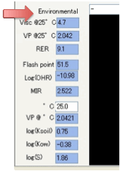
The Viscosity at 25ºC is estimated. This is
a very difficult parameter to estimate and the
values should be seen only as a guide. This output was requested by a number of
customers who said that they were happy with an indicative value. Vapour
Pressure @ 25ºC
is a useful guide to the relative volatility of a compound though you can also
enter a ºC parameter and get the vapour pressure at
that temperature too. From the vapour pressure, the RER (Relative Evaporation Rate, nBuAc=100) is estimated via the
empirical formula RER=0.046*MVol*VapourPressure. The Flash Point estimate is handy to know if your
chemical will fall in the wrong domain for your application. The Carter MIR value is an objective measure of the
ability of the Volatile Organic Compound to react with ozone,
and the Log[OH] value is an estimate of the rate of
reaction with the .OH radical. When you combine the chemical knowledge from the
HSP with the relative volatility and reactivity estimates you gain a powerful
insight into possible substitutions for your current (high VOC) chemistry.
The default is for just the HSP and MVol
to be placed onto the Clipboard for pasting (Ctrl-P) into other HSP fields or
for going into Excel etc.
If you would like the full set of data on
the Clipboard, select Full data to
Clipboard.
After the calculation the data (with
headings) is easily pasted into, say, Excel.
So it’s very easy to use – provided you
have your molecule in one of the formats that Y-MB can read (Smiles, .mol,
.mol2, .xyz, .pdb, .gpr). It’s generally easy to find Smiles or .mol for a
molecule. You can also enter your molecule into any of the common (and often
free) molecular drawing packages which will give you output in one of these
formats). You can also use Open Babel (which is free) to convert from one
format (such as InChI) to another. It would be nice to have InChI format as an
input, but it is rather complex so it is easier for us to ask you to use Open
Babel. For those who (for various reasons) don’t have molecular drawing
packages and don’t like to risk revealing structures to on-line drawing tools,
the Draw2SMILES Power Tool is simple
but powerful.
As a bonus, when you load one of the 3D
file formats (Load 3D), you can check that the molecule is
what you think it is with a simple 3D viewer.
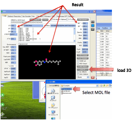
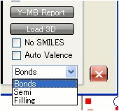
The bonds can be shown as Bonds, Semi, or Filling depending on your choice.
You can of course 3D rotate the molecule
and Zoom (Shift-Click) or Pan (Ctrl-Click). The 3D technique is identical to
that used in viewing the Sphere.
There are two options when using Load 3D.
The first is No SMILES. This bypasses the
built-in SMILES generator and for complex molecules can produce a considerable
increase in speed in generating the HSP values. The second is an Auto Valence option. Some 3D files omit hydrogens and
omit information as to whether a bond is single, double or triple. If you
select the Auto Valence option, the program does its best to estimate the
degree of the bond, without which Y-MB cannot function properly. This is
particularly important for aromatic molecules where an alternating
single-double pattern has to be created. It’s impossible for Auto Valence to be
right all the time. It’s far better if you provide the 3D information with all
hydrogens and bond-orders specified. But sometimes Auto Valence is better than
nothing and just occasionally it makes matters worse. Use your discretion!
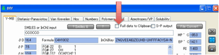
If you have a large set of compounds in
Smiles format, you can use Y-MB to File
Convert
them into a standard .hsd file and a .sof (Optimizer) file. The file format
(.txt or .bat) is very easy. For each chemical you need a Name, a Smiles and,
optionally, a CAS No in that order. Each column is separated by a Tab (so you
can, if you wish, create this from within Excel as “Tab separated format”). The
file can, optionally, include a first line saying Name, Smiles, CAS – though
this line will then be ignored.
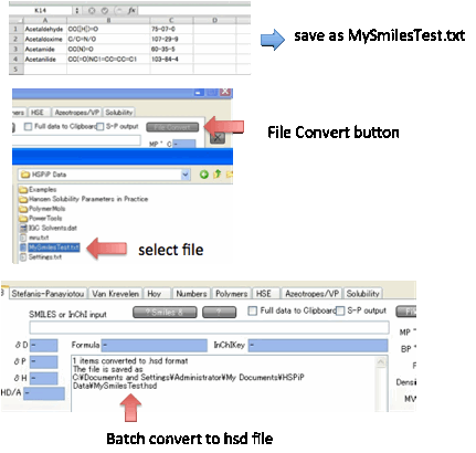
If all goes well, the converted file will
have the same name as the original but with .hsd (and, separately, .sof)
instead of .txt or .dat. You can then load it straight into HSPiP. If Y-MB
fails to convert a molecule it will be shown in the .hsd file but all the
values will be empty. The line will be missing from the .sof file.
If you select the S-P Output option then the Y-MB routine also
calculates the Stefanis-Panayiotou UNIFAC first-order groups for you and places
them in the S-P tab.
There are, unfortunately, some
limitations to this so please don’t accept the S-P output as being 100% true.
In our experience it is usually more reliable than a normal chemist who doesn’t
handle UNIFAC groups every day, but it can still make some mistakes.
The Y-MB method is a powerful source of
other information.
If it thinks that it recognises the
functionality in your Smiles input it will list the molecules in HSPiP Solvent
Data that have identical functionality – along with the actual HSP. If you find
that the Y-MB estimate is very wrong, you can click on the Y-MB Report button, enter the values you think are
the correct ones, click the Put
report on Clipboard button and past your report into your email program and
send it to steve@hansen-solubility.com.
As you might be interested in other
molecules with similar functionality, the Y-MB
Analogs
button creates a list of molecules (+HSP) which contain the functionality of
your molecule.
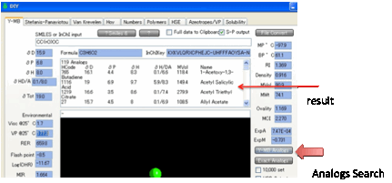
This can be quite a long list. If you
want just the functionality in your target
molecule then click Exact Analogs for a more exclusive
list. We find this functionality amazingly helpful as a source of ideas for
alternative formulations and for problem solving. The list you create is
automatically placed on the Clipboard in a format that is easy to paste into
Excel. If you want the list as a .hsd file that’s then automatically imported
into HSPiP, check the HSD Output option.
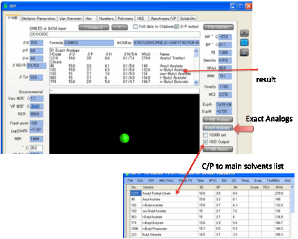
You can choose to search in the standard
HSP list or by checking the 10K (short for 10,000)
option, the entire database.
Although Y-MB provides a long list of
parameters, even more are available in the Y-Predict Power Tool. Whilst
there is no plan to increase the range of predictions for HSPiP, Y-Predict will
continue to expand, depending on user needs and Hiroshi’s own research
interests.
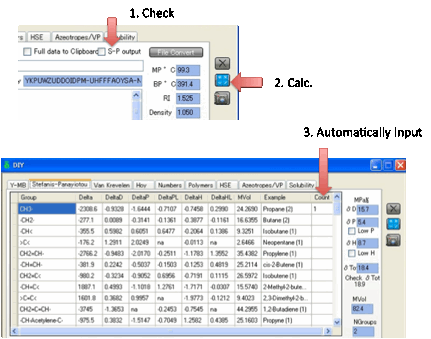
3 Stefanis-Panayiotou
Stefanis and Panayiotou have produced a
sophisticated group-contribution method for calculating δD, δP, δH, δTot and Molar Volume. All you have to do
is break down your molecule into its component groups and enter how many of
each group are in your molecule. For example, 1-Butanol possesses 1 CH3- group,
3 –CH2- groups and 1 –OH group.
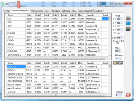
If you enter the numbers for 1-Butanol
and press the Calculate button you get the calculated values of 21.9 for δTot. The other values are compared to
Hansen’s table.
δD δP δH MVol
Calculated 15.9 6.1 13.2 94.3
Hansen 16.0 5.7 15.8 91.5
There is also another Check δTot value calculated from the individual δD, δP and δH values which you can compare to the
estimated δTot.
For a molecule such as 1-Butanol it’s
easy to know how to break it down. For more complex molecules you need help.
The first strength of the Stefanis-Panayiotou method is that the break-down
uses the standard UNIFAC method and you will find numerous other examples in
the literature of molecules being broken down in this manner. The second
strength is that they have helpfully provided examples in their table that make
it easy to work out the appropriate substructures.
Stefanis and Panayiotou recognised the
fundamental flaw in the simple group contribution method – that, for example, 3
–CH2- groups behave very differently depending on whether they are part of
1-Butanol or cyclobutanol.
So they have added a further refinement.
In addition to the 1st-order table, there is a 2nd-order
table with important sub-structures. With a bit of practice you can quickly
determine which 2nd-order contributions to include. By selecting
them, the results for more complex molecules are more accurate.
It’s worth noting that δP and δH contribution methods must be less accurate than δD. The reason is simple. δD mostly depends heavily on how much
“stuff” you have in the molecules. But δP and δH depend crucially on configuration which
cannot simply be captured in a table of group contributions. As a further aid
for this issue, if you suspect that the true δP and/or δH values of your molecule should be low,
clicking the LowP and/or LowH option gives you values
correlated especially for this scenario and therefore likely to be more
accurate.
The authors of the technique stress that
the technique is designed to be used with molecules with more than 3 carbon
atoms or 3 functional groups. So although the program allows you to calculate
the value for, say, methanol or ethanol, the results are not accurate. In
practice this is not a limitation as HSP for such simple molecules are likely
to be known already.
You might like to save your group
assignments for reference, or for changing your mind later on. Click the Save button and the group assignments are saved as a .spg
(Stefanis-Panayiotou Group) file. The Open button retrieves the
group assignments from your chosen file.
To learn more of the S-P methodology,
consult their paper on δTot
and δD:
E. Stefanis, L. Constantinou, C.
Panayiotou; A Group-Contribution Method for
Predicting Pure Component Properties of Biochemical and Safety Interest; Ind. Eng. Chem. Res.
2004, 43, 6253-6261
Their work on δP and δH is included in:
Physical
and Chemical Parameters of Paper Conservation, PhD thesis by
Emmanuel Stefanis (In Greek), Department
of Chemical Engineering,
Aristotle University of Thessaloniki,
Greece, 2007 and the full paper in International Journal of Thermophysics is
found in:
Emmanuel Stefanis, Costas Panayiotou, Prediction of Hansen Solubility Parameters with a New
Group-Contribution Method, International Journal of Thermophysics, 2008 , 29
(2), 568-585.
The parameters and equations used in this
version differ slightly from those in the published work. Dr Stefanis kindly
re-ran the correlations using the most up-to-date version of the HSP table.
This, happily, removed many/most of the outliers shown in the Internationl
Journal of Thermophysics paper and improved the correlation coefficients.
The Y-MB method allows you the option
automatically to create (or at least produce a good estimate of) the S-P UNIFAC
(first-order) groups. There are some known imperfections (e.g. a lack of
pyridine groups) so use the results with caution.
4 Van Krevelen
Van Krevelen also admits that group
contribution techniques cannot be expected to be accurate. But they are
certainly better than nothing. Once again, you simply identify which groups
make up your molecule and enter the number of each group. No 2nd-order
effects are included.
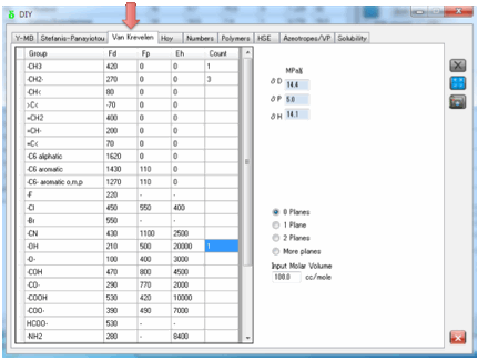
You need to input a Molar Volume – see
item (1) for how you might obtain this.
You also need to specify if you have
multiple planes of symmetry. The more symmetry, the less polar effect there is
(0.5 for 1 plane, 0.25 for 2 planes) and if you have 3 planes then both the
polar and hydrogen bonding values are set to 0.
5 Hoy
Hoy’s approach is more complex and it
attempts to take into account many more factors.
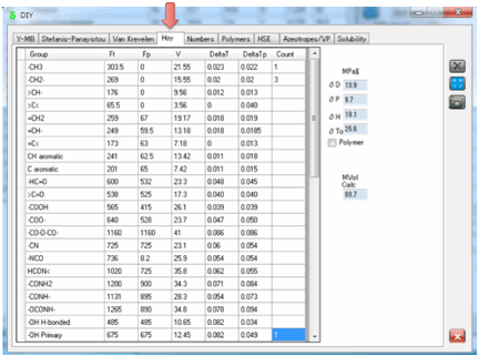
For example, there is a Polymer mode which takes into account the fact
that values calculated for your simple repeat unit are unlikely to apply to the
polymer itself. Hoy also assigns a partial molar volume to each group so you
end up with an estimate of the molar volume as part of the calculation.
Remember to never mix Hoy values with other values – his scheme, whilst excellent,
is based on a different partition of δTot. So it is self-consistent but not
consistent with other methods.
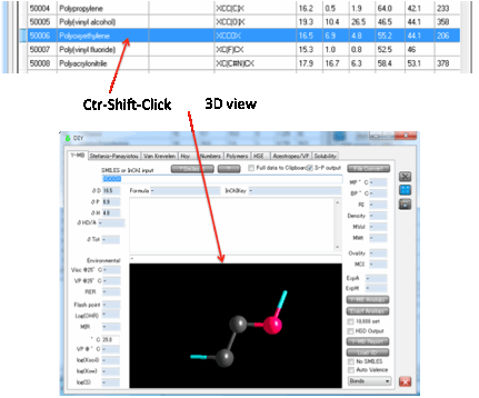
6 Polymers
As an adjunct to the Y-MB method we have
introduced Polymer Y-MB. In earlier editions this took (with his kind
permission) the vast data table generously provided by Dr W. Michael Brown at
Sandia National Laboratories.
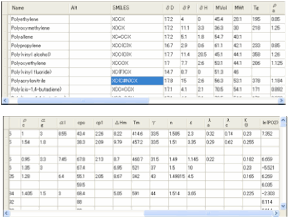
For the 3rd Edition we
increased the number of polymers to >600 and used an –X notation instead of
the original “cyclic 0” nomenclature of Dr Brown. This has allowed us more
versatility and also allowed us to correct a number of errors in the Smiles
nomenclature in the original database. Double click (or Alt-click) on any of
those polymers and the Smiles is put into the box, click on Calculate and the
Polymer Smiles estimate is produced.
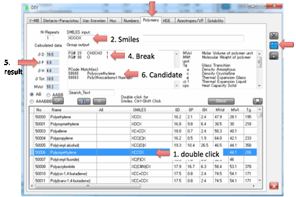
If you Ctrl-Click on a polymer then the
tab changes to Y-MB where the 3D viewer shows you the monomer unit, with the
dangling bonds clearly visible.
You can also calculate the Polymer Y-MB
from this tab. If you set the N-Repeats to more than 1 then an
n-mer Smiles is created and the Y-MB values calculated.
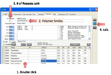
The calculated HSP change for different
n-mers. This is because the science of predicting polymer-HSP is not yet
robust, though it is greatly improved thanks to the new techniques in the 3rd
Edition. At this stage (as with any HSP predictions) you have to use your
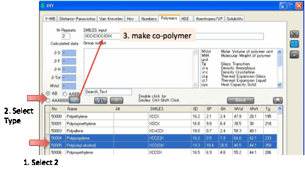
judgement. You can enter Polymer Smiles by hand. You can also create AB, AABB
or AAABBB polymers by selecting two monomer rows, clicking the appropriate
selection then clicking the CP (Co-Polymer) button.
If your own polymer isn’t in the table
you can create your own Smiles string. For complicated molecules, such as a
cellulose derivative, it’s difficult to create the Smiles string accurately
yourself. One way to do this to create the molecule in a standard molecular
drawing package, using something like Br to show where the polymer chain goes:
The package can then automatically
provide you with the Smiles string for this pseudo-molecule:
OC1C(OC)C(OC(COCCC)C1Br)OBr
Now all you need to do is replace the two
Br atoms with the X for polymer Smiles
OC1C(OC)C(OC(COCCC)C1X)OX
This can go straight into Y-MB or the
Polymer tab and you get your predicted HSP values.
The Draw2Smiles Power Tool allows you
to enter a polymer structure in a simple chemical drawing program, add the
Polymer “atoms” at the appropriate places and calculate a Polymer SMILES that
can be pasted (Ctrl-C) into the text box. This can also be used as a quick way
to find a polymer within the table. If the Polymer SMILES results in a match to
one of the polymers in the table, this is shown in the output box.
For those who make more complex polymer
blends there is a simple Blend option. Select 2 or
more monomers from the table, click the Blend option and enter the % of each
monomer, then click the Calculate button to obtain your estimate.
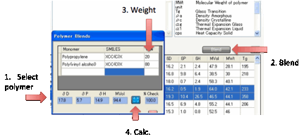
Clearly this is very limited. It assumes
a random blend of your components (i.e. a reactivity ratio of 1 for each
monomer) and determines the statistical blend of AA, AB, AC, BB, BC, CC (for a
3-component blend) diads and from their calculated HSP values and their
volume-weighted (not mass weighted!) values obtains the final result. Such
predictions need to be treated with due caution.
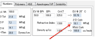
δD from tables
The δD parameter can also be found with the
charts given in the second edition of the Handbook. This requires knowledge or
estimate of the critical temperature. At the same time it could be noted that
this procedure is a corresponding states calculation, CST, (in agreement with
the Prigogine CST approach), and that this could be the basic reason for some
differences in the group contribution methods.
Why no Beerbower table?
The Hansen handbook is honest about the
limitations of the group contribution approach. The Beerbower values included
in the handbook show wide error bars and it would not do justice to the table
to simply include some fixed value. In addition, the table does not cover as
wide a range of groups as the other methods. However, in the hands of an
expert, the table can be valuable and users might find it instructive to derive
their own estimates manually.
Which method is the best?
Only you can tell. The calculator is
called DIY because you really do have to do it yourself. You are a scientist,
so use your judgement. If the values of one approach don’t make sense when you
compare them to a similar molecule for which you already know the value, then
see if a different approach gives you a value which seems more reasonable. The
Stefanis-Panayiotou method (2007) is based on a large data set using modern
statistical techniques, is a method published in the literature and uses the
much-used UNIFAC sub-structures so is a good choice. The Y-MB method is highly
convenient because it takes you automatically from structure to HSP and the
neural network and multiple-regression parameters have been trained on the
entire HSP dataset provided with HSPiP so many users will find that it gives
helpful results. In addition it also provides lots more parameter estimates. So
it is our favourite. But in the end, use your own judgement.
Other
predictions
Using the Y-MB method it is possible to
obtain many predicted values. These can be used in many ways, described in this
section.
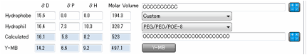
Surfactants
On the Numbers
& Surfactants tab,
you have the ability to create HSP for your surfactant of choice. This is done
by providing a set of hydrophils and a set of hydrophobes.
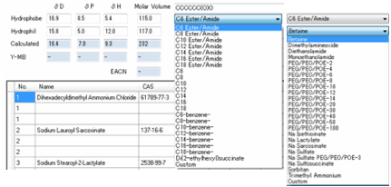
The idea is that you “mix and match” with
whatever is the closest approximation to your desired surfactant. This is a
relatively crude method, but the calculated values are a useful starting point
that you can refine for your own purposes. The calculated value is the weighted
average of the two components, based on their relative molar volumes. If you
don’t like the pre-assigned values, you can enter your own HSP parameters and
molar volumes into the respective boxes and the weighted average calculation is
carried out for you.
SC Johnson have generously allowed us to
use their table of surfactant HSP (calculated for them by Dr Hansen) which
might give you an alternative way of estimating the values for your own
specific surfactants. You can sort the table by HLB (Hydrophilic-Lipophilic
Balance) or by type (Anionic, Cationic etc.) for your convenience.
As an alternative, the Y-MB button
automatically generates a SMILES input to the Y-MB calculator and returns the
HSP values.
This only works when Y-MB has relevant
data. A number of the hydrophilic headgroups are undefined in SMILES terms so
for these the Y-MB calculation is automatically disabled and a message appears
to explain why.
You can also customize either the head or
tail via your own SMILES string. This allows you greater versatility. Enter a
SMILES then press the calculate button next to it and it will be added to the
simple head + tail calculator. You can also click the Y-MB button to calculate
the full molecule, though for large molecules this is very slow and not too
satisfactory.
For those familiar with HLD-NAC
surfactant theory (see AbbottApps for an app-based explanation) it is important
to know the Effective Alkane Carbon Number (EACN) of the oil.
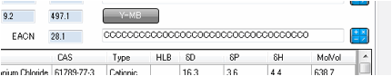
This can be estimated from the SMILES of
your chosen oil.
HSE (Health, Safety and Environment)
Decisions on which solvents/chemicals to
use are seldom simple. Trade-offs have to be made with cost, VOCs, toxicity,
environmental impact and so forth. To make rational decisions, it’s good to
have side-by-side comparisons of key, relevant properties. That’s what the HSE
tab does. Enter two chemicals (as SMILES) and click the Calculate button.
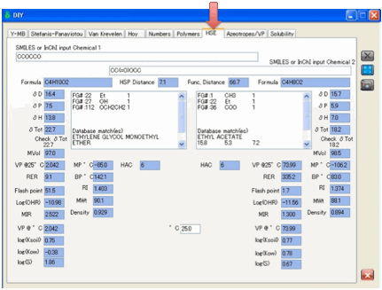
In addition to standard properties such
as molecular weight, molar volume, density, melting point, boiling point,
properties provided include:
Vapour Pressure (at 25º, at specified
temperature and in terms of Antoine Constants)
RER – Relative
Evaporation Rate (n-Bu Acetate=100)
Log(OHR) – the OH
radical reactivity
MIR – the Carter MIR
measure of VOC activity
Log(Ksoil) – the
soil/water partition coefficient
Log(Kow) – the
octanol/water partition coefficient
Log(S) – the water
solubility
Furthermore there are two numerical
estimates of similarity. In both cases values closer to zero mean greater
similarity.
HSP Distance – the
Distance in HSP space
Functional Distance – a
measure of the difference in functional groups between the two molecules.
These two numbers are very helpful in
“read across” estimation in, for example, REACH.
Azeotropes and Vapour Pressures
If you can estimate the activity
coefficients of two chemicals and if you know (or can estimate) their vapour
pressures as pure liquids, then it is possible to calculate the vapour
pressures of the two chemicals above the liquid. You can do this in two ways
Calculating the vapour
pressures of the two components at various mole fractions at a temperature of
interest
Calculating the vapour
pressures at the boiling point of the mixture across the mole fraction range.
The first calculation is the classic
vapour-pressure equilibrium curve. The second enable the classic calculation of
Azeotropes.
To perform these calculations, simply
enter the SMILES of the two chemicals and click Calculate.
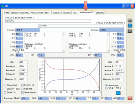
This gives estimated values for boiling
points, vapour pressures, Antoine Coefficients and also gives two numbers, the
so-called Margules parameters, which allow the activity coefficients for the
two chemicals to be calculated across the whole mole fraction range.
If you don’t like the estimates, you can
always manually enter values for the key parameters and click the local
Calculate button to update the graph.
The plots offer a lot of choice. The
first choice is between Vapour Pressures and Azeotropes. If the latter is
chosen then the full Azeotrope data are provided as outputs: Mole fraction,
Weight % and Volume % and boiling point of the Azeotrope (if it exists), and
the HSP of the Azeotrope.
The graphs include options to
Show the ideal curves so you can visually
check the deviation from ideality
Show the 0-1 lines which simply show what
would happen if the liquids were ideal and had the same vapour pressure –
again, just as a visual reference
Show the Azeotrope boiling point, in ºC (disabled for the
Vapour Pressures plot)
Plot X1, X2 means that the graphs for
both liquids start with 0 at the left-hand origin. Conventionally, X1 is
plotted in this manner, with X2 plotted with 0 in the right-hand origin. Use
whichever you find more comfortable and informative
Plot Wt% - use a Wt% scale rather than
(the conventional) mole fraction scale.
Show Gamma – plots the activity
coefficients of the two liquids over the range. You cannot plot Temperature and
Gamma on the same graph.
Feel free to use as many or as few of
these options as give you the information you want.
When you move your mouse over the graph,
you get a readout of the relevant properties at that point.
Solubility
It seems odd to say that you cannot
directly predict solubility from HSP! But HSP have always been about relative
solubility and have never attempted to issue exact solubility predictions.
However, with some simple equations and
some good estimations of key properties, it is possible to predict solubilities
directly.
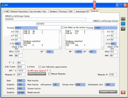
The equation is simple:
Ln(Solubility) = – C + E – A – H
C is the “Crystalline” term. It is the
Van ‘t Hoff (or Prausnitz) formula that depends on the difference between the
current temperature, T, and the melting point Tm, the Gas Constant R
and also on the Enthalpy of Fusion DeltaF.
C = DeltaF/R*(1/Tm – 1/T)
In other words, the higher the melting
point and the higher the enthalpy of fusion, the more difficult it is to
transform the solid into the dissolved (liquid) state.
This formula is a simplification which
follows convention and ignores some other terms like heat capacities.
For calculations where Tm<T,
C is set to zero. The calculations start to become meaningless in this
liquid/liquid scenario, but it seems instructive to carry out the calculation.
A warning is provided to alert you to the problem.
The E term is (combinatorial) Entropy.
This is calculated from volume fractions (Phi) and molar volumes.
E = 0.5*PhiSolvent*(VSolute/VSolvent
-1) + 0.5*ln(PhiSolute + PhiSolvent*VSolute/VSolvent)
It’s worth making an important reminder
that molar volumes for solids are not based on their
molecular weight and solid density. In the words
of Ruelle: “(For a solid) the molar volume to consider is not that of the pure
crystalline substance but the volume of the substance in its hypothetical
subcooled liquid state.”
A comes from the activity coefficient.
The larger the activity coefficient, the more negative A becomes. A simple
estimate of activity coefficient comes from the HSP distance – not
surprisingly, the larger the distance, the higher the activity coefficient and
the lower the solubility. Because the simple HSP distance has been shown to be
only an approximate guide to activity coefficients, the Margules coefficient
predictor from the Azeotropes and Vapour Pressures calculator is used. Molar
volumes play a significant role in activity coefficients, so a large molecule
with similar HSP values is significantly less soluble than a smaller one.
H is a Hydrophobic Effect term that is
very important for solublities in water, and somewhat important for
solubilities in low alcohols. The calculation follows the method of Ruelle and
depends on PhiSolvent*VSolute/VSolvent with
extra terms depending on how many hydrogen-bond donors (alcohols, phenols,
amines, amides, thiols) are on the solute and whether the solvent is water, a
mono-alcohol or a poly-ol. If the solvent is water and the solute contains
alcohol groups, there are special parameters depending on whether the alcohols
are primary, secondary or tertiary. There is a further refinement (not included
in this version) which discounts some of the solute’s hydrogen bond donors if
they are likely to be internally bonded.
The complication is that the E, A and H
terms all depend on the volume or molar fraction which is the precisely what
you are trying to calculate, so there is an iterative process involved till the
equation balances.
The output is the Ideal solubility (as
mole fraction), the real solubility (as mole fraction, volume fraction and
weight %) plus the following (which come from taking the exponential of their
terms in the log-solubility equation):
The ideal solubility is divided by the Activity coefficient. For ideal
solutes this is 1. For moderately soluble chemicals it is in the range 1 to 10,
for highly incompatible solutes it can rise to more than 100.
The ideal solubility is multiplied by the Entropy term. This is usually
larger than 1, except for small solutes in large solvents.
The ideal solubility is multiplied by the Hydrophobic term. This is usually
less than 1 for large molecules in water or typical alcohols. It is 1 for
non-water/alcohol solvents.
From these four terms you get a very good
idea of where the solubility or insolubility is coming from.
Because water is such a special solvent,
click the Use Water as the solvent option for the solvent
rather than enter [H]O[H] into the solvent SMILES box. Because both the
entropic and hydrophobic effects in water are so large, don’t expect the
calculation to be amazingly accurate for solubilities below 0.05 mole fraction.
At this stage there aren’t good Margules parameter estimates so they are both
set to 0 (ideal!) and you’ll need to make your own judgement of what they
should be. A warning label appears to remind you of this fact.
Because the predictions of HSP, MPt and
Margules are all subject to error, feel free to override any/all of them and
re-calculate solubility using the Manual
Calculation
button.
For those interested in the theory, the Solubility Theory button opens a form where the effects of
MPt, Enthalpy of Fusion, Delta Heat Capacity, Heat of Mixing and Entropy of
Mixing can all be explored, as well as the simple Yalkowsky assumption. The
graph (which can be read with the mouse) plots the mole fraction solubility v
temperature, with 0°C being the lowest temperature and the MPt being the
highest temperature. Alternatively the data can be shown as a van’t Hoff plot
of ln(x) v 1/T where the ideal case is a straight line shown in black as a
reference.
Solubility is increased (i.e. you get a
higher mole fraction at a lower temperature) with a lower MPt, a lower Enthalpy
of Fusion, a higher Delta Heat Capacity and a negative Heat of Mixing. The
theory is explained in the eBook. Note that at some positive values of Heat of
Mixing the curve takes on an odd shape. For reasons explained in the eBook
these curves are unrealistic (they violate the Gibbs phase rules) and instead
represent “oiling out” phenomena.